- Главная
- Разное
- Дизайн
- Бизнес и предпринимательство
- Аналитика
- Образование
- Развлечения
- Красота и здоровье
- Финансы
- Государство
- Путешествия
- Спорт
- Недвижимость
- Армия
- Графика
- Культурология
- Еда и кулинария
- Лингвистика
- Английский язык
- Астрономия
- Алгебра
- Биология
- География
- Детские презентации
- Информатика
- История
- Литература
- Маркетинг
- Математика
- Медицина
- Менеджмент
- Музыка
- МХК
- Немецкий язык
- ОБЖ
- Обществознание
- Окружающий мир
- Педагогика
- Русский язык
- Технология
- Физика
- Философия
- Химия
- Шаблоны, картинки для презентаций
- Экология
- Экономика
- Юриспруденция
Lemke’s Algorithm: The Hammer in Your Math Toolbox? презентация
Содержание
- 1. Lemke’s Algorithm: The Hammer in Your Math Toolbox?
- 2. First, a Word About Hammers requirements for
- 3. Hammers (cont.) by definition, not the optimal
- 4. What are “advanced game math problems”? problems
- 5. Prerequisites linear algebra vector, matrix symbol manipulation
- 6. Overview of Lecture random assortment of example
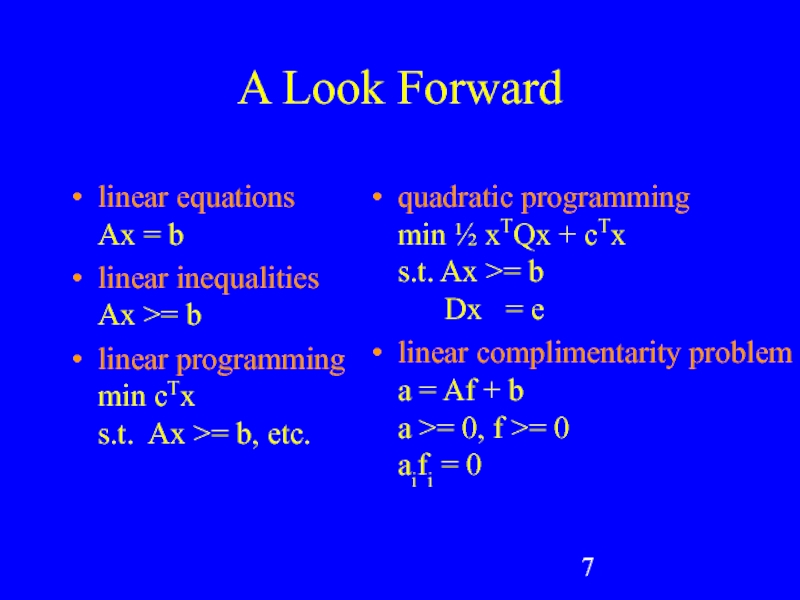
- 7. A Look Forward linear equations Ax =
- 8. Applications to Games graphics, physics, ai, even
- 9. Applications to Games (cont.) don’t forget...
- 10. Specific Examples #1a: Ease Cubic Fitting
- 11. Specific Examples #1a: Ease Cubic
- 12. Specific Examples #1a: Ease Cubic
- 13. Specific Examples #1a: Ease Cubic
- 14. Specific Examples #1b: Cubic Spline Fitting
- 15. Specific Examples #1b: Cubic Spline Fitting
- 16. Specific Examples #2: Minimum Cost Network
- 17. Specific Examples #2: Minimum Cost Network
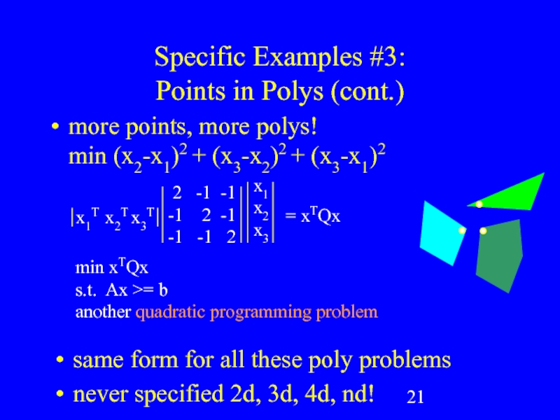
- 18. Specific Examples #3: Points in
- 19. Specific Examples #3: Points in
- 20. Specific Examples #3: Points in Polys
- 21. Specific Examples #3: Points in Polys
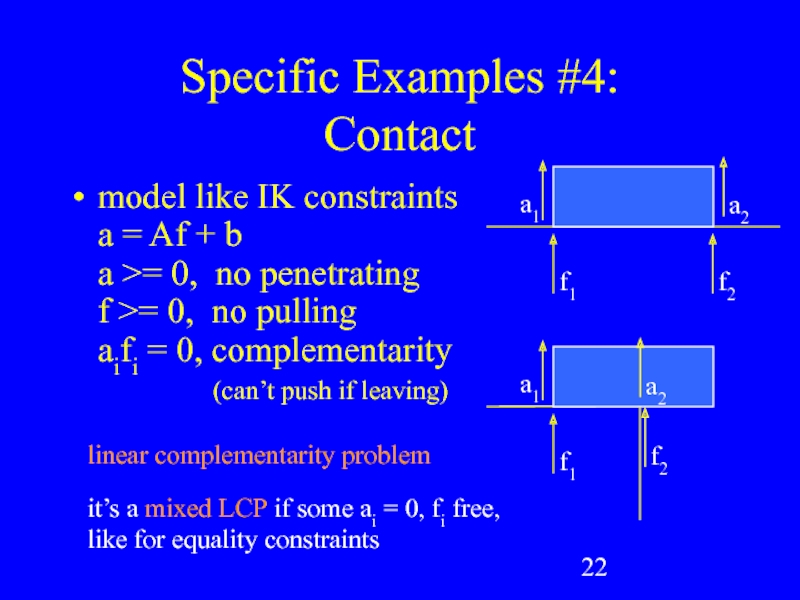
- 22. Specific Examples #4: Contact model like
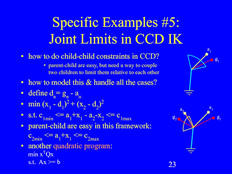
- 23. Specific Examples #5: Joint Limits in
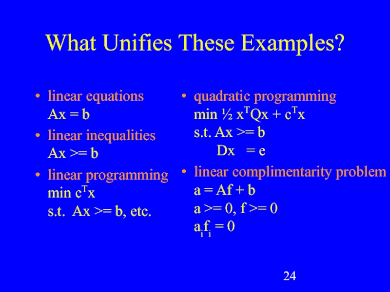
- 24. What Unifies These Examples? linear equations Ax
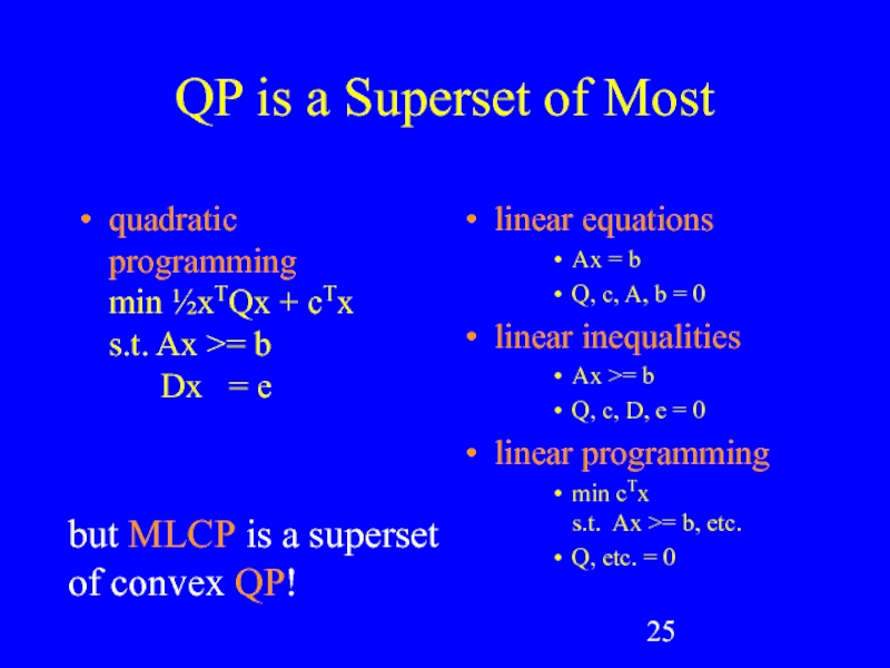
- 25. QP is a Superset of Most quadratic
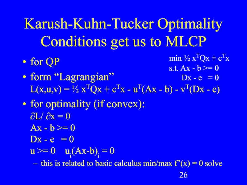
- 26. Karush-Kuhn-Tucker Optimality Conditions get us to MLCP
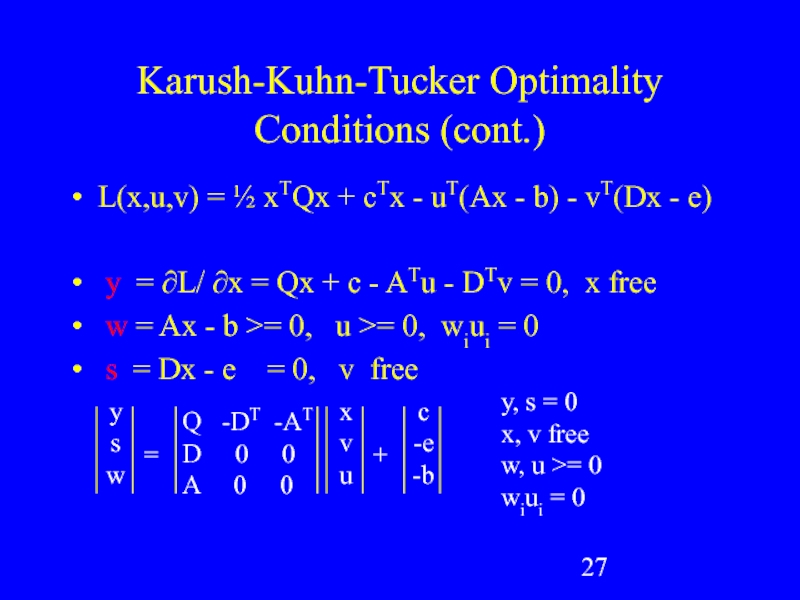
- 27. Karush-Kuhn-Tucker Optimality Conditions (cont.) L(x,u,v) = ½
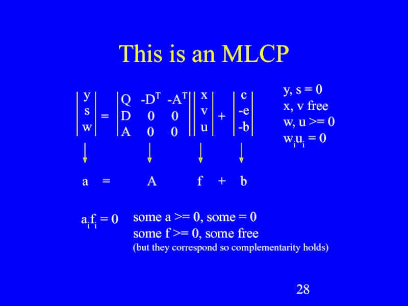
- 28. This is an MLCP x v u
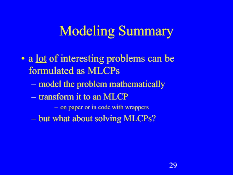
- 29. Modeling Summary a lot of interesting problems
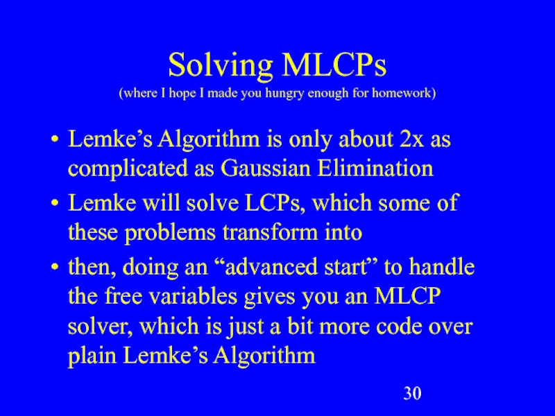
- 30. Solving MLCPs (where I hope I made
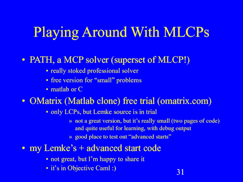
- 31. Playing Around With MLCPs PATH, a MCP
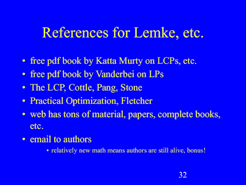
- 32. References for Lemke, etc. free pdf book
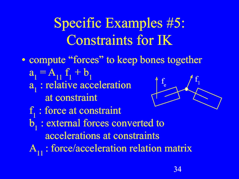
- 34. Specific Examples #5: Constraints for IK
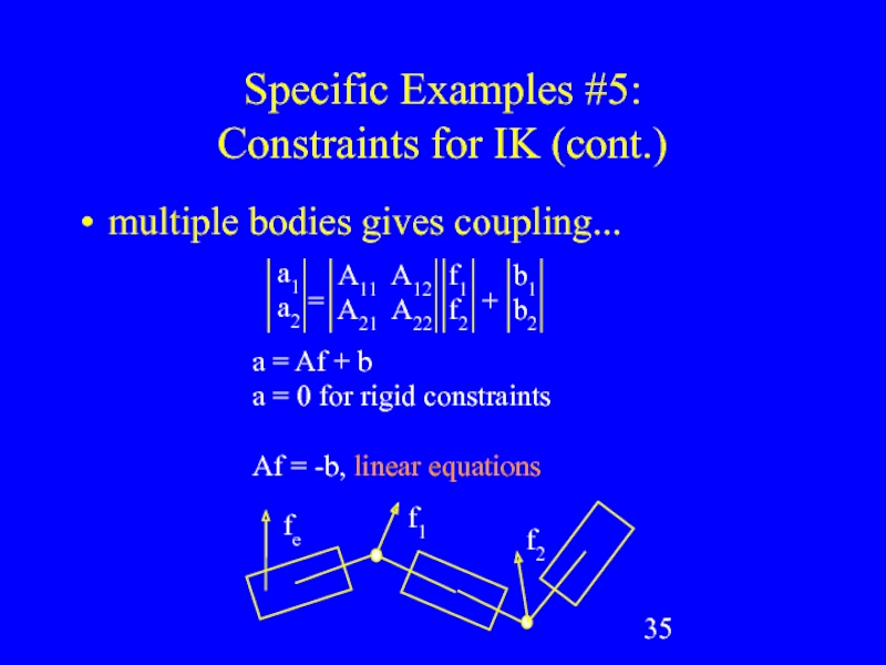
- 35. Specific Examples #5: Constraints for IK
Слайд 1Lemke’s Algorithm:
The Hammer in Your Math Toolbox?
Chris Hecker
definition six, inc.
checker@d6.com
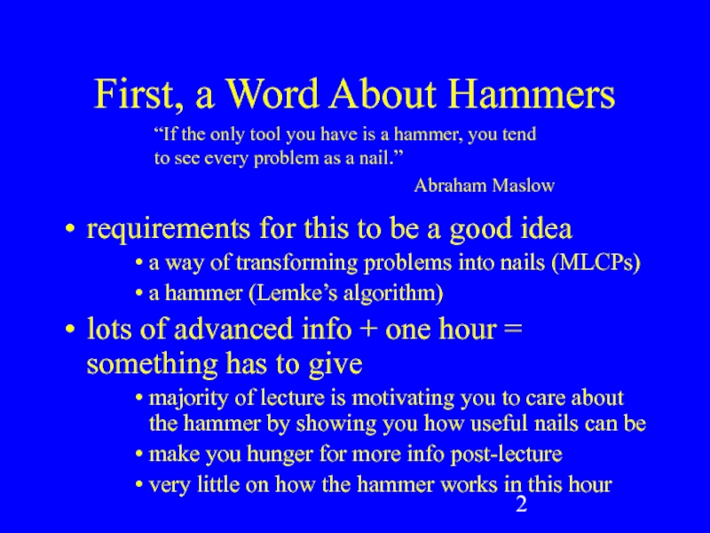
Слайд 2First, a Word About Hammers
requirements for this to be a good
a way of transforming problems into nails (MLCPs)
a hammer (Lemke’s algorithm)
lots of advanced info + one hour = something has to give
majority of lecture is motivating you to care about the hammer by showing you how useful nails can be
make you hunger for more info post-lecture
very little on how the hammer works in this hour
“If the only tool you have is a hammer, you tend to see every problem as a nail.”
Abraham Maslow
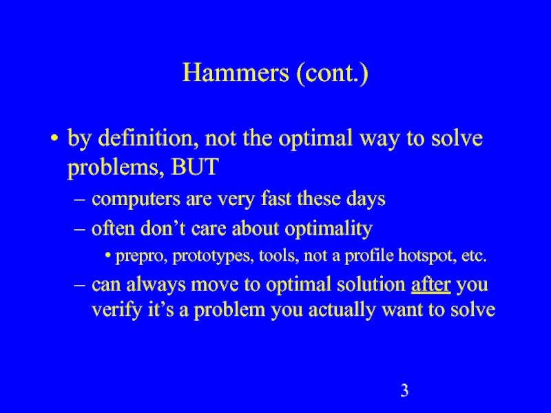
Слайд 3Hammers (cont.)
by definition, not the optimal way to solve problems, BUT
computers
often don’t care about optimality
prepro, prototypes, tools, not a profile hotspot, etc.
can always move to optimal solution after you verify it’s a problem you actually want to solve
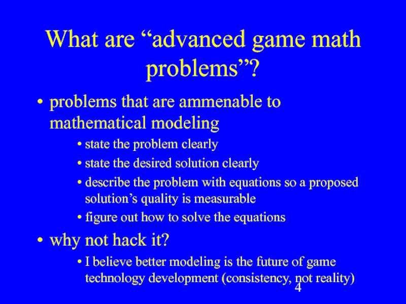
Слайд 4What are “advanced game math problems”?
problems that are ammenable to mathematical
state the problem clearly
state the desired solution clearly
describe the problem with equations so a proposed solution’s quality is measurable
figure out how to solve the equations
why not hack it?
I believe better modeling is the future of game technology development (consistency, not reality)
Слайд 5Prerequisites
linear algebra
vector, matrix symbol manipulation at least
calculus concepts
what derivatives mean
comfortable with
Слайд 6Overview of Lecture
random assortment of example problems breifly mentioned
5 specific example
including one that I ran into recently and how I solved it
generalize the example models
transform them all to MLCPs
solve MLCPs with Lemke’s algorithm
Слайд 7A Look Forward
linear equations
Ax = b
linear inequalities
Ax >= b
linear programming
min
quadratic programming
min ½ xTQx + cTx
s.t. Ax >= b
Dx = e
linear complimentarity problem
a = Af + b
a >= 0, f >= 0
aifi = 0
Слайд 8Applications to Games
graphics, physics, ai, even ui
computational geometry
visibility
contact
curve fitting
constraints
integration
graph theory
network flow
economics
site
game theory
IK
machine learning
image processing
Слайд 9Applications to Games (cont.)
don’t forget...
The Elastohydrodynamic Lubrication Problem
Solving Optimal Ownership Structures
“The
Слайд 10Specific Examples #1a:
Ease Cubic Fitting
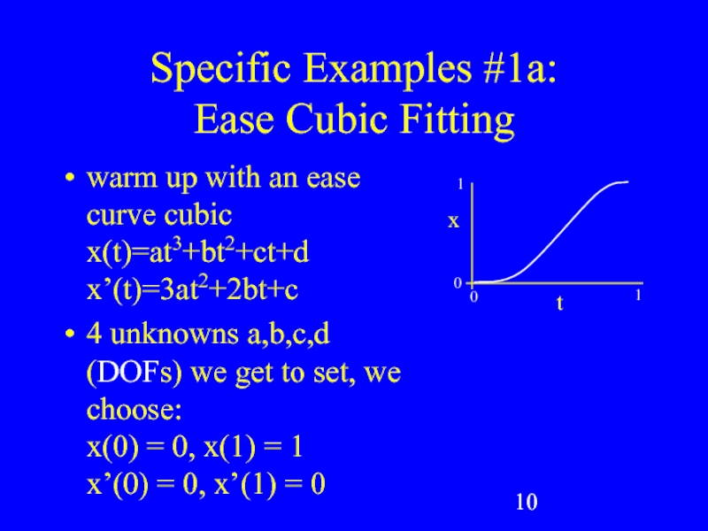
warm up with an ease curve
4 unknowns a,b,c,d (DOFs) we get to set, we choose: x(0) = 0, x(1) = 1 x’(0) = 0, x’(1) = 0
1
x
t
0
0
1
Слайд 11Specific Examples #1a:
Ease Cubic Fitting (cont.)
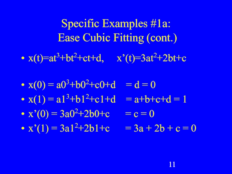
x(t)=at3+bt2+ct+d, x’(t)=3at2+2bt+c
x(0)
x(1) = a13+b12+c1+d = a+b+c+d = 1
x’(0) = 3a02+2b0+c = c = 0
x’(1) = 3a12+2b1+c = 3a + 2b + c = 0
Слайд 12Specific Examples #1a:
Ease Cubic Fitting (cont.)
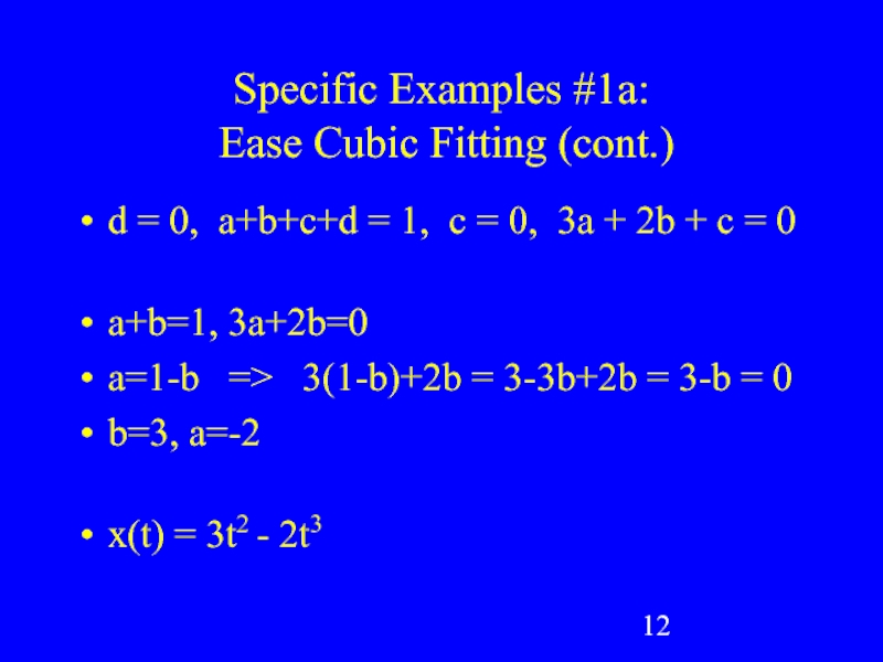
d = 0, a+b+c+d
a+b=1, 3a+2b=0
a=1-b => 3(1-b)+2b = 3-3b+2b = 3-b = 0
b=3, a=-2
x(t) = 3t2 - 2t3
Слайд 13Specific Examples #1a:
Ease Cubic Fitting (cont.)
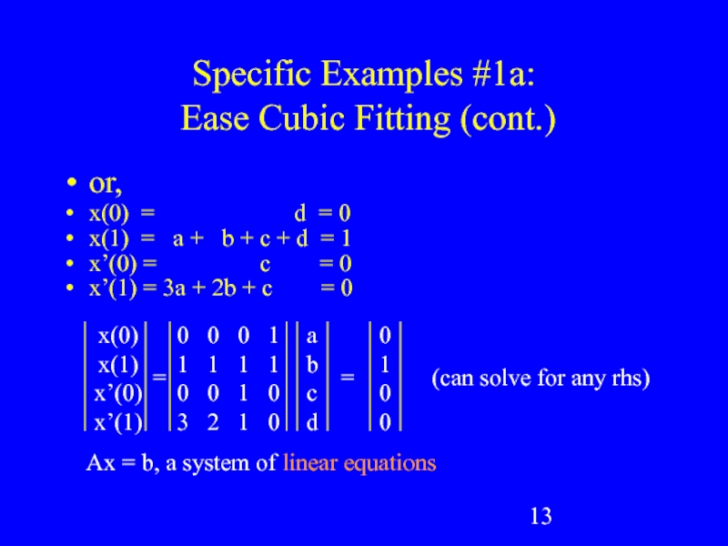
or,
x(0) =
x(1) = a + b + c + d = 1
x’(0) = c = 0
x’(1) = 3a + 2b + c = 0
0 0 0 1
1 1 1 1
0 0 1 0
3 2 1 0
x(0)
x(1)
x’(0)
x’(1)
a
b
c
d
0
1
0
0
=
=
Ax = b, a system of linear equations
(can solve for any rhs)
Слайд 14Specific Examples #1b:
Cubic Spline Fitting
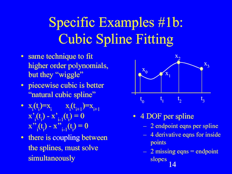
same technique to fit higher order
piecewise cubic is better “natural cubic spline”
xi(ti)=xi xi(ti+1)=xi+1 x’i(ti) - x’i-1(ti) = 0 x’’i(ti) - x’’i-1(ti) = 0
there is coupling between the splines, must solve simultaneously
x0
x1
x2
x3
t0
t1
t2
t3
4 DOF per spline
2 endpoint eqns per spline
4 derivative eqns for inside points
2 missing eqns = endpoint slopes
Слайд 15Specific Examples #1b:
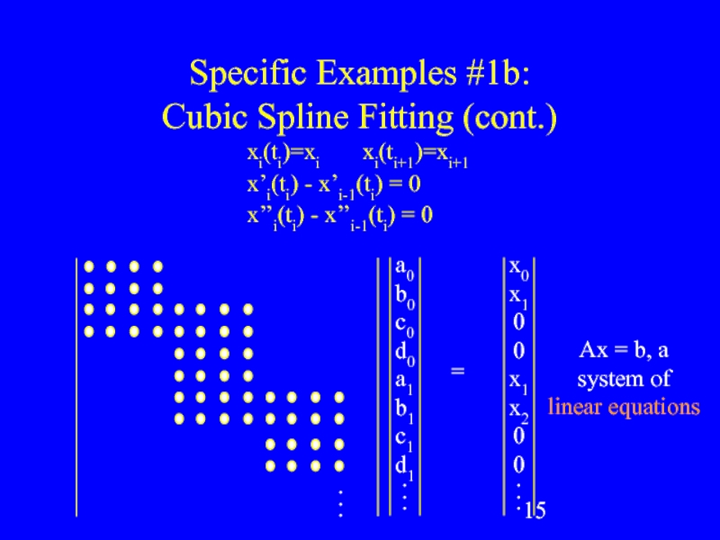
Cubic Spline Fitting (cont.)
a0
b0
c0
d0
a1
b1
c1
d1
.
.
.
x0
x1
0
0
x1
x2
0
0
.
.
.
=
xi(ti)=xi xi(ti+1)=xi+1
x’i(ti)
.
.
.
Ax = b, a system of
linear equations
Слайд 16Specific Examples #2:
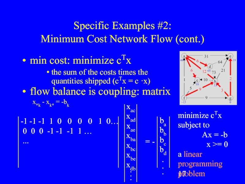
Minimum Cost Network Flow
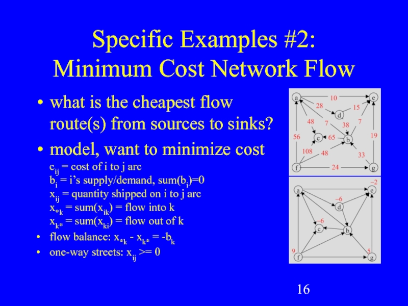
what is the cheapest flow
model, want to minimize cost cij = cost of i to j arc bi = i’s supply/demand, sum(bi)=0 xij = quantity shipped on i to j arc x*k = sum(xik) = flow into k xk* = sum(xki) = flow out of k
flow balance: x*k - xk* = -bk
one-way streets: xij >= 0
Слайд 17Specific Examples #2:
Minimum Cost Network Flow (cont.)
min cost: minimize cTx
the
flow balance is coupling: matrix x*k - xk* = -bk
xac
xad
xae
xba
xbc
xbe
xdb
.
.
.
= -
-1 -1 -1 1 0 0 0 0 1 0…
0 0 0 -1 -1 -1 1 …
...
ba
bb
bc
bd
.
.
.
minimize cTx
subject to
Ax = -b
x >= 0
a linear programming problem
Слайд 18
Specific Examples #3:
Points in Polys
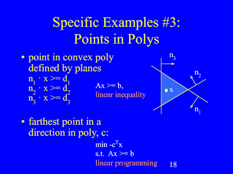
point in convex poly defined by
farthest point in a direction in poly, c:
n1
n2
n3
x
Ax >= b,
linear inequality
min -cTx
s.t. Ax >= b
linear programming
Слайд 19
Specific Examples #3:
Points in Polys (cont.)
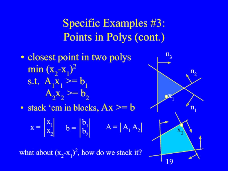
closest point in two polys
min
stack ‘em in blocks, Ax >= b
n1
n2
x1
n3
x2
x1
x2
x =
A1 A2
A =
what about (x2-x1)2, how do we stack it?
b1
b2
b =
Слайд 20Specific Examples #3:
Points in Polys (cont.)
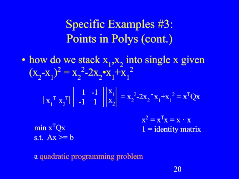
how do we stack x1,x2
x1
x2
x1T x2T
1 -1
-1 1
= x22-2x2 • x1+x12 = xTQx
min xTQx
s.t. Ax >= b
a quadratic programming problem
x2 = xTx = x · x
1 = identity matrix
Слайд 21Specific Examples #3:
Points in Polys (cont.)
more points, more polys!
min (x2-x1)2
x1
x2
x3
x1T x2T x3T
2 -1 -1
-1 2 -1
-1 -1 2
min xTQx
s.t. Ax >= b
another quadratic programming problem
same form for all these poly problems
never specified 2d, 3d, 4d, nd!
= xTQx
Слайд 22Specific Examples #4:
Contact
model like IK constraints
a = Af + b
a
f1
f2
a1
a2
f1
f2
a1
a2
linear complementarity problem
it’s a mixed LCP if some ai = 0, fi free, like for equality constraints
Слайд 23Specific Examples #5:
Joint Limits in CCD IK
how to do child-child
parent-child are easy, but need a way to couple two children to limit them relative to each other
how to model this & handle all the cases?
define dn= gn - an
min (x1 - d1)2 + (x2 - d2)2
s.t. c1min <= a1+x1 - a2-x2 <= c1max
parent-child are easy in this framework: c2min <= a1+x1 <= c2max
another quadratic program: min xTQx s.t. Ax >= b
a1
g1
a2
g2
a1
g1
Слайд 24What Unifies These Examples?
linear equations
Ax = b
linear inequalities
Ax >= b
linear
quadratic programming
min ½ xTQx + cTx
s.t. Ax >= b
Dx = e
linear complimentarity problem
a = Af + b
a >= 0, f >= 0
aifi = 0
Слайд 25QP is a Superset of Most
quadratic programming
min ½xTQx + cTx
s.t. Ax
linear equations
Ax = b
Q, c, A, b = 0
linear inequalities
Ax >= b
Q, c, D, e = 0
linear programming
min cTx
s.t. Ax >= b, etc.
Q, etc. = 0
but MLCP is a superset of convex QP!
Слайд 26Karush-Kuhn-Tucker Optimality Conditions get us to MLCP
for QP
form “Lagrangian”
L(x,u,v) = ½
for optimality (if convex): ∂L/ ∂x = 0 Ax - b >= 0 Dx - e = 0 u >= 0 ui(Ax-b)i = 0
this is related to basic calculus min/max f’(x) = 0 solve
min ½ xTQx + cTx
s.t. Ax - b >= 0
Dx - e = 0
Слайд 27Karush-Kuhn-Tucker Optimality Conditions (cont.)
L(x,u,v) = ½ xTQx + cTx - uT(Ax
y = ∂L/ ∂x = Qx + c - ATu - DTv = 0, x free
w = Ax - b >= 0, u >= 0, wiui = 0
s = Dx - e = 0, v free
x
v
u
Q -DT -AT
D 0 0
A 0 0
=
y
s
w
+
c
-e
-b
y, s = 0
x, v free
w, u >= 0
wiui = 0
Слайд 28This is an MLCP
x
v
u
Q -DT -AT
D 0
A 0 0
=
y
s
w
+
c
-e
-b
y, s = 0
x, v free
w, u >= 0
wiui = 0
a
=
A
f
b
+
aifi = 0
some a >= 0, some = 0
some f >= 0, some free
(but they correspond so complementarity holds)
Слайд 29Modeling Summary
a lot of interesting problems can be formulated as MLCPs
model
transform it to an MLCP
on paper or in code with wrappers
but what about solving MLCPs?
Слайд 30Solving MLCPs
(where I hope I made you hungry enough for homework)
Lemke’s
Lemke will solve LCPs, which some of these problems transform into
then, doing an “advanced start” to handle the free variables gives you an MLCP solver, which is just a bit more code over plain Lemke’s Algorithm
Слайд 31Playing Around With MLCPs
PATH, a MCP solver (superset of MLCP!)
really stoked
free version for “small” problems
matlab or C
OMatrix (Matlab clone) free trial (omatrix.com)
only LCPs, but Lemke source is in trial
not a great version, but it’s really small (two pages of code) and quite useful for learning, with debug output
good place to test out “advanced starts”
my Lemke’s + advanced start code
not great, but I’m happy to share it
it’s in Objective Caml :)
Слайд 32References for Lemke, etc.
free pdf book by Katta Murty on LCPs,
free pdf book by Vanderbei on LPs
The LCP, Cottle, Pang, Stone
Practical Optimization, Fletcher
web has tons of material, papers, complete books, etc.
email to authors
relatively new math means authors are still alive, bonus!
Слайд 34Specific Examples #5:
Constraints for IK
compute “forces” to keep bones together
a1
f1
fe
Слайд 35Specific Examples #5:
Constraints for IK (cont.)
multiple bodies gives coupling...
a1
a2
A11 A12
A21
f1
f2
b1
b2
=
+
f1
f2
fe
a = Af + b
a = 0 for rigid constraints
Af = -b, linear equations
