Random variables – discrete random variables. Week 6 (2) презентация

variables

DR SUSANNE HANSEN SARAL
EMAIL: SUSANNE.SARAL@OKAN.EDU.TR
HTTPS://PIAZZA.COM/CLASS/IXRJ5MMOX1U2T8?CID=4#
WWW.KHANACADEMY.ORG

DR SUSANNE HANSEN SARAL

will occur, is not known, therefore the word “random”.

DR SUSANNE HANSEN SARAL

Ch. 4-

Random
Variables

Discrete
Random Variable

Continuous
Random Variable

outcome from a random experiment.
It takes on countable values, integers.

Examples of discrete random variables:
Number of cars crossing the Bosphorus Bridge every day
Number of journal subscriptions
Number of visits on a given homepage per day

We can calculate the exact probability of a discrete random variable:

values. Therefore called continuous random variable

Continuous random variables are common in business applications for modeling physical
quantities such as height, volume and weight, and monetary quantities such as profits, revenues
and expenses.

Examples:
The weight of cereal boxes filled by a filling machine in grams
Air temperature on a given summer day in degrees Celsius
Height of a building in meters
Annual profits in $ of 10 Turkish companies

values.

The probability of a continuous variable is calculated in an interval (ex.: 5 -10), because the probability of a specific continuous random variable is close to 0. This would not provide useful information.

Example: The time it takes for each of 110 employees in a factory to assemble a toaster:

Time, in seconds, it takes 110 employees to assemble a toaster

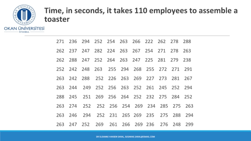
271 236 294 252 254 263 266 222 262 278 288
262 237 247 282 224 263 267 254 271 278 263
262 288 247 252 264 263 247 225 281 279 238
252 242 248 263 255 294 268 255 272 271 291
263 242 288 252 226 263 269 227 273 281 267
263 244 249 252 256 263 252 261 245 252 294
288 245 251 269 256 264 252 232 275 284 252
263 274 252 252 256 254 269 234 285 275 263
263 246 294 252 231 265 269 235 275 288 294
263 247 252 269 261 266 269 236 276 248 299

DR SUSANNE HANSEN SARAL, SUSANNE.SARAL@GMAIL.COM

time in seconds

Completion time (in seconds) Frequency Relative frequency %
220 – 229 5 4.5
230 – 239 8 7.3
240 – 249 13 11.8
250 – 259 22 20.0
260 – 269 32 29.1
270 – 279 13 11.8
280 – 289 10 9.1
290 – 300 7 6.4
Total 110 100 %

DR SUSANNE HANSEN SARAL, SUSANNE.SARAL@GMAIL.COM

Models

For both discrete and continuous variables, the collection of all possible outcomes (sample space) and probabilities associated with them is called the probability model.

For a discrete random variable, we can list the probability of all possible values in a table.
For example, to model the possible outcomes of a dice, we let X be the random variable called the “number showing on the face of the dice”. The probability model for X is therefore:

1/6 if x = 1, 2, 3, 4, 5, or 6
P(X = x) =
0 otherwise

Variables

Let X be a discrete random variable and x be one of its possible values

The probability that random variable X takes specific value x is denoted P(X = x).
In the dice example: X is the random variable “the number showing on the
dice” and it’s value, x = the specific number. Ex.: P( X = 3)

The probability distribution function, P(x) of a random variable, X, is a representation of the probabilities for all the possible outcomes, x.

The function can be shown algebraically, graphically, or with a table:

Probability Distributions Function, P(x) for Discrete Random Variables

0 1/4 = .25
1 2/4 = .50
2 1/4 = .25

Experiment: Toss 2 Coins simultaneously. Let the random variable, X, be the # heads

T

T

4 possible outcomes (values for x)

T

T

H

H

H

H

Probability Distribution

0 1 2 x

.50
.25

Probability

for Discrete Random Variables (example)

Sales of sandwiches in a sandwich shop:
Let, the random variable X, represent the number of sandwiches sold within the time period of 14:00 - 16:00 hours in one given day. The probability distribution function, P(x) of sales is given by the table here below:

DR SUSANNE HANSEN SARAL

probability distribution of sandwich sales between 14:00 -16:00 hours

DR SUSANNE HANSEN SARAL

a probability distribution of a discrete random variable

DR SUSANNE HANSEN SARAL

Ch. 4-

1. 0 ≤ P(x) ≤ 1 for any value of x

2. The individual probabilities of all outcomes sum up to 1;





All possible values of X are mutually exclusive and collectively exhaustive (the outcomes make up the entire sample space), therefore the probabilities for these events must sum to 1.

P(x) F(x)
0 0.25 0.25
1 (x2) 0.50 0.75
2 0.25 1.00

Example: Toss 2 coins simultaneously
Let the random variable, X, be number of the heads. There are 4 possible outcomes:

P(x) F(x0)
A 0.18 0.18 = 0.18
B 0.32 0.50 = 0.18 + 0.32
C 0.25 0.75 = 0.50 + 0.25
D 0.07 0.82 = 0.75 + 0.07
E 0.03 0.85 = 0.82 + 0.03
F 0.15 1.00 = 0.85 + 0.15

Example: Let the random variable, X, be the grades obtained in a geography exam and x = A, B, C, D, E, F are the possible outcomes/values :

the random variable, X, be the grades obtained in a geography exam.

Cumulative probability distribution, Ogive

DR SUSANNE HANSEN SARAL

Ch. 4-

Example: Let the random variable, X, be the grades obtained in a geography exam.

Practical application

DR SUSANNE HANSEN SARAL

The cumulative probability distribution can be used for example for inventory planning?


Based on an analysis of it’s sales history, the manager of a car dealer knows that on any single day the number of Toyota cars sold can vary from 0 to 5.

Practical application: Car dealer

DR SUSANNE HANSEN SARAL

The random variable, X, is the number of possible cars sold in a day:

Practical application

DR SUSANNE HANSEN SARAL

Example: If there are 3 cars in stock. The car dealer will be able to satisfy 85% of the customers

Practical application

DR SUSANNE HANSEN SARAL

Example: If only 2 cars are in stock, then 35 % [(1-.65) x 100]
of the customers will not have their needs satisfied.

variable X. It has been found that students have the following probabilities of getting a specific grade:
A: .18 D: .07
B: .32 E: .03
C: .25 F: .15
Based on this, calculate the following:
The cumulative probability distribution of X, F(x)
The probability of getting a higher grade than B
The probability of getting a lower grade than C
The probability of getting a grade higher than D
The probability of getting a lower grade than B

DR SUSANNE HANSEN SARAL

probability distribution of X, F(x0)
The probability of getting a higher grade than B, P(x > B)
The probability of getting a lower grade than C, P(x < C)
The probability of getting a grade higher than D P(x > D)
The probability of getting a lower grade than B P(x < B)

DR SUSANNE HANSEN SARAL

for discrete random variables:

Expected value E[X] of a discrete random variable - expectations

Expected Variance of a discrete random variable

Expected Standard deviation of a discrete random variable

Why do we refer to expected value?

DR SUSANNE HANSEN SARAL

random variable, X = # of heads,

(TT, HT,TH,HH) compute the expected value of X:

DR SUSANNE HANSEN SARAL

Ch. 4-

x P(x)
0 .25
1 .50
2 .25

Value (or mean) of a discrete random variable X:




We weigh the possible outcomes by
the probabilities of their occurrence:

E(x) = (0 x .25) + (1 x .50) + (2 x .25) = 1.0

DR SUSANNE HANSEN SARAL

Ch. 4-

x P(x)
0 .25
1 .50
2 .25

value, E[X], of a discrete random variable is found by multiplying each possible value of the random variable by the probability that it occurs and then summing all the products:



The expected value of tossing two coins simultaneously is therefore:

E[x] = (0 x .25) + (1 x .50) + (2 x .25) = 1.0

textbooks reveals that 81 % of the pages have no mistakes, 17 % of
the pages have one mistake and 2% have two mistakes.

We use the random variable X to denote the number of mistakes on a page chosen at random
from a textbook with possible values, x, of 0, 1 and 2 mistakes.

With a probability distribution of :
P(0) = .81 P(1) = .17 P(2) = .02

How do we calculate the expected value(average) of mistakes per page?

DR SUSANNE HANSEN SARAL

on pages:


= (0)(.81)+(1)(.17)+(2)(.02) =.21

From this result we can conclude that over a large number of pages, the expectation would be to find an average of 21 % mistakes per page in business textbooks.

DR SUSANNE HANSEN SARAL

HANSEN SARAL

for $ 3 each. If the biggest prize is $ 250 and 4 second prizes are $ 50 each :

a) What are the possible outcomes?
b) What is the expected value, E[X], of a single ticket?
c) Now, include the cost of the ticket you bought. What is the expected value now?
d) Knowing the value calculated in part b) does it make sense to buy a lottery ticket?
e) What is the expected value the lottery company can expect to gain from the lottery
sale?

for $ 3 each. If the biggest prize is $ 250 and 4 second prizes are $ 50 each.

a) What are the possible outcomes? Winning the large prize of $ 250, 1/500, winning one of the 4
prizes of $ 50, 4/500 and winning nothing, $ 0, 495/500
b) What is the expected value, E[X], of a single ticket?
E[X] = $ 250 x (1/500) + $ 50x (4/500) + $ 0 x (495/500) = $ 0.50 +$ 0.40 +$ 0.00 = $ 0.90
c) Now, include the cost of the ticket you bought. What is the expected value now?
E[X] = $ 0.90 - $ 3.00 = $ - 2.10
d) Knowing the value calculated in part b) does it make sense to buy a lottery ticket?

lose $ 2.10, because they either lose $3 or win $ 250 or $ 50.

$ 2.10 is the amount in average that the lottery organization gains per ticket.

The lottery can therefore expect to make 500 x $ 2.10 = $ 1050 by selling 500 lottery tickets.