1. Non-stationary random walk trajectories modeling
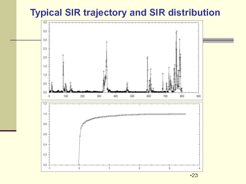
2. SIR Indicator trajectory
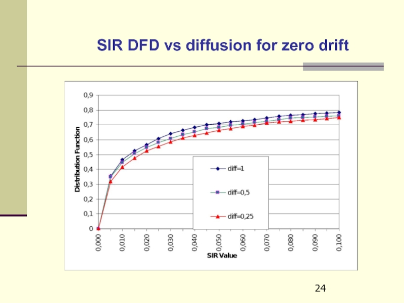
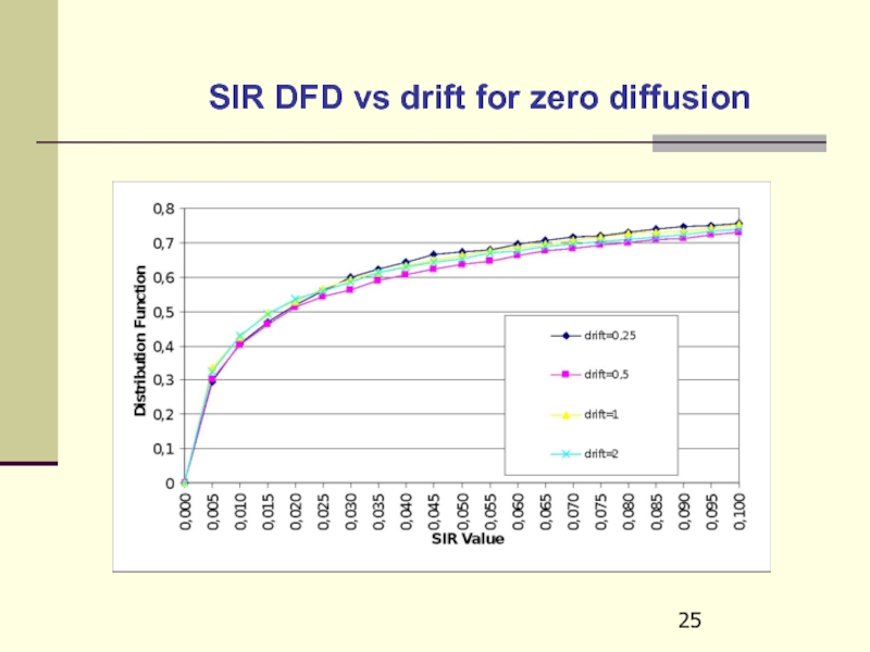
3. Distribution of SIR Indicator
4. Distribution of the first break down moment
5. Cashing effects
- Главная
- Разное
- Дизайн
- Бизнес и предпринимательство
- Аналитика
- Образование
- Развлечения
- Красота и здоровье
- Финансы
- Государство
- Путешествия
- Спорт
- Недвижимость
- Армия
- Графика
- Культурология
- Еда и кулинария
- Лингвистика
- Английский язык
- Астрономия
- Алгебра
- Биология
- География
- Детские презентации
- Информатика
- История
- Литература
- Маркетинг
- Математика
- Медицина
- Менеджмент
- Музыка
- МХК
- Немецкий язык
- ОБЖ
- Обществознание
- Окружающий мир
- Педагогика
- Русский язык
- Технология
- Физика
- Философия
- Химия
- Шаблоны, картинки для презентаций
- Экология
- Экономика
- Юриспруденция
D2D wireless connection modeling for moving devices in 5G technology презентация
Содержание
- 1. D2D wireless connection modeling for moving devices in 5G technology
- 2. The problem in general
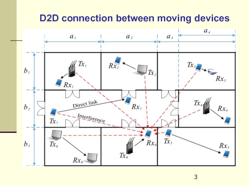
- 3. D2D connection between moving devices
- 4. The main steps of modeling 1. Construction
- 5. Generation of non-stationary trajectories of random walk
- 6. Kinetic approach Let the distribution
- 7. Correctness of Fokker-Planck Equation for Empirical Distribution
- 8. Explicit scheme
- 9. Typical
- 10. Probability Density Evolution Model
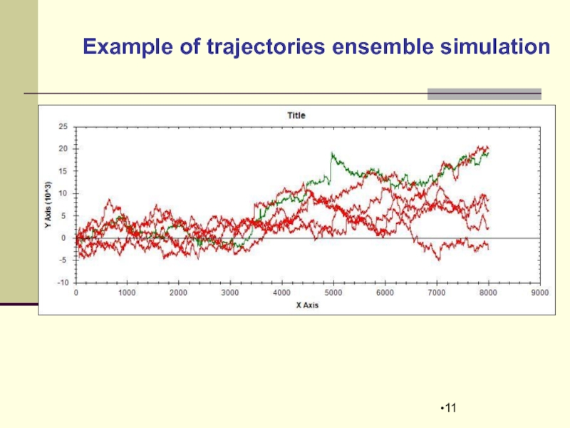
- 11. Example of trajectories ensemble simulation
- 12. For any given
- 13. Correctness of ensemble generation Initially
- 14. SIR Indicator Trajectory
- 15. SIR value in a continuous media From
- 16. Example
- 17. Let us derive the evolution equation for
- 18. Final
- 19. SIR dispersion evolution equation – 1
- 20. SIR dispersion evolution equation – 2
- 21. Stability D2D connection indicator
- 22. SIR Indicator Distribution Function
- 23. Typical SIR trajectory and SIR distribution
- 24. SIR DFD vs diffusion for zero drift
- 25. SIR DFD vs drift for zero diffusion
- 26. Analysis of D2D connection stability
- 27. The SIR standard deviation We consider
- 28. Indicator of stability We consider two
- 29. The SIR Simulation The
- 30. Distribution Function of the first break down moment
- 31. Simulation
- 32. Classical
- 33. Simulation
- 34. Analysis of cashing effects
- 35. Simulation results for DFD first break down
- 36. Empirical dependence of the maximum continuity period
- 37. The type of normalized DFD
- 38. Conclusions Numerical simulation the SIR
- 39. The
- 40. THANK YOU FOR
Слайд 1
Sergey L. Fedorov
Keldysh Institute of Applied Mathematics of RAS
D2D wireless connection
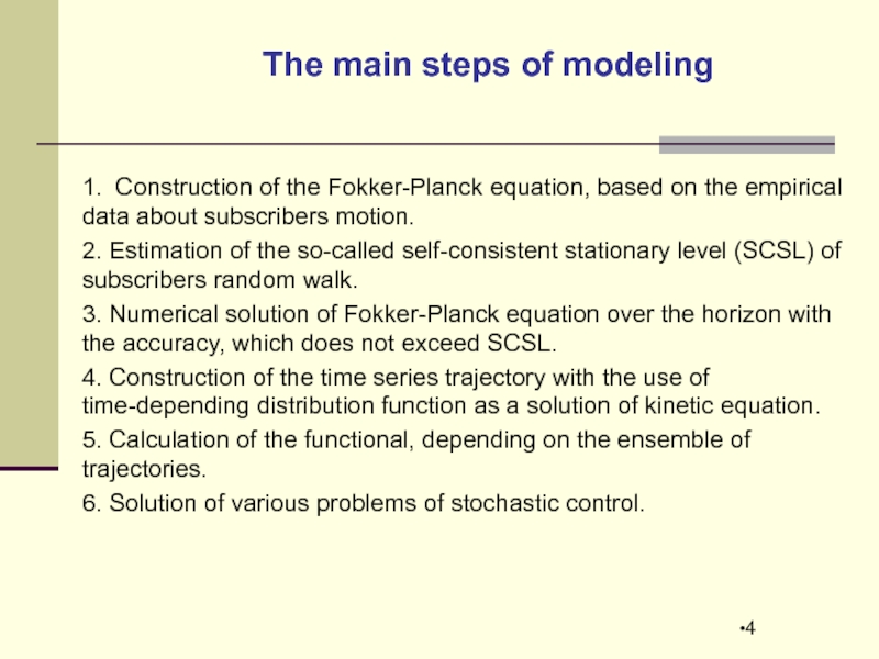
Слайд 4The main steps of modeling
1. Construction of the Fokker-Planck equation, based
2. Estimation of the so-called self-consistent stationary level (SCSL) of subscribers random walk.
3. Numerical solution of Fokker-Planck equation over the horizon with the accuracy, which does not exceed SCSL.
4. Construction of the time series trajectory with the use of time-depending distribution function as a solution of kinetic equation.
5. Calculation of the functional, depending on the ensemble of trajectories.
6. Solution of various problems of stochastic control.
Слайд 6Kinetic approach
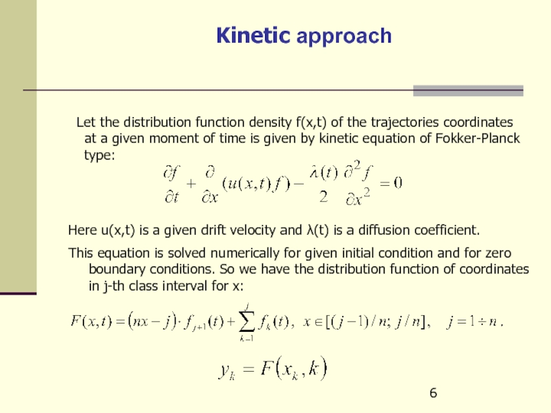
Let the distribution function density f(x,t) of the
Here u(x,t) is a given drift velocity and λ(t) is a diffusion coefficient.
This equation is solved numerically for given initial condition and for zero boundary conditions. So we have the distribution function of coordinates in j-th class interval for x:
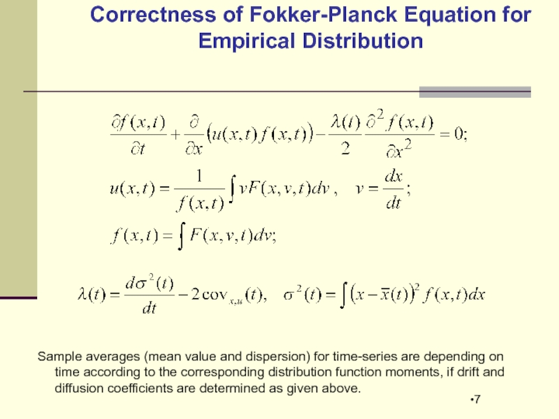
Слайд 7Correctness of Fokker-Planck Equation for Empirical Distribution
Sample averages (mean value
Слайд 8
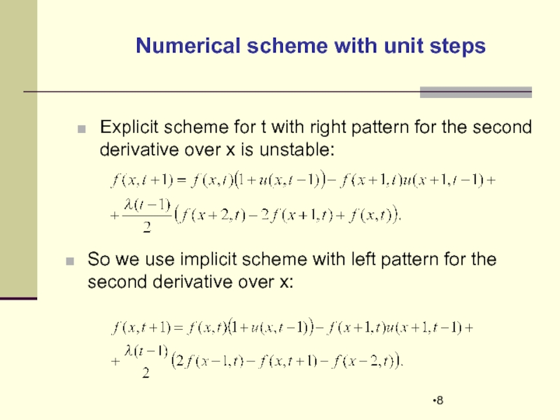
Explicit scheme for t with right pattern for the second derivative
So we use implicit scheme with left pattern for the second derivative over x:
Numerical scheme with unit steps
Слайд 9
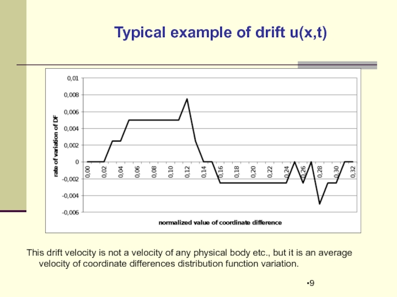
Typical example of drift u(x,t)
This drift velocity is not
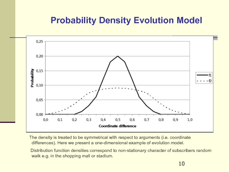
Слайд 10Probability Density Evolution Model
The density is treated to
Distribution function densities correspond to non-stationary character of subscribers random walk e.g. in the shopping mall or stadium.
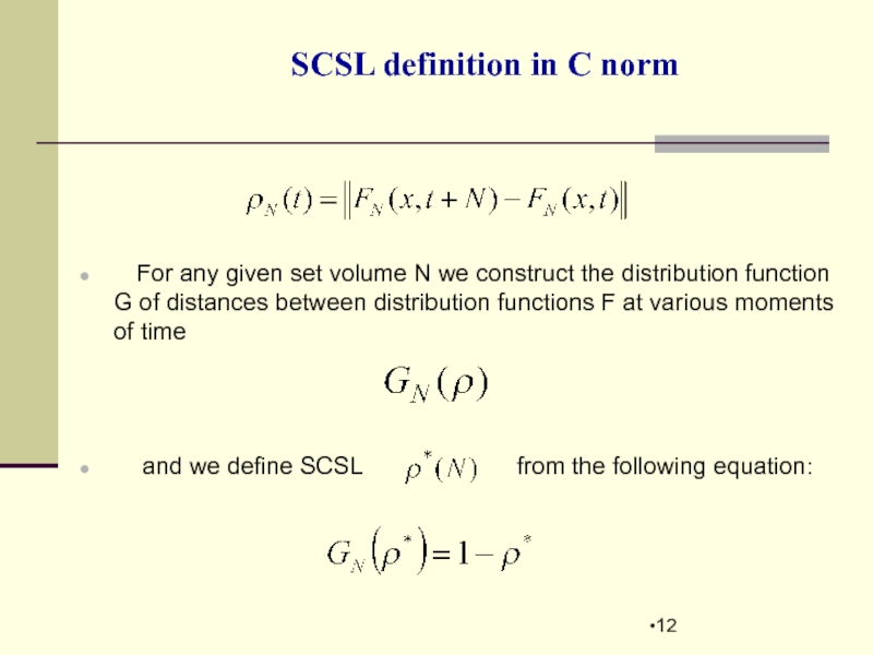
Слайд 12
For any given set volume N we construct the
and we define SCSL from the following equation:
SCSL definition in C norm
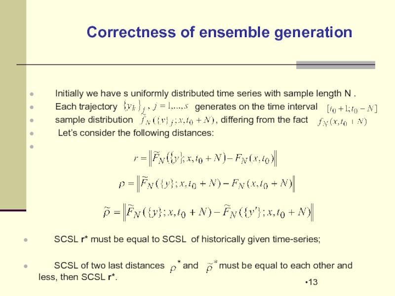
Слайд 13Correctness of ensemble generation
Initially we have s uniformly distributed
Each trajectory generates on the time interval
sample distribution , differing from the fact
Let’s consider the following distances:
SCSL r* must be equal to SCSL of historically given time-series;
SCSL of two last distances and must be equal to each other and less, then SCSL r*.
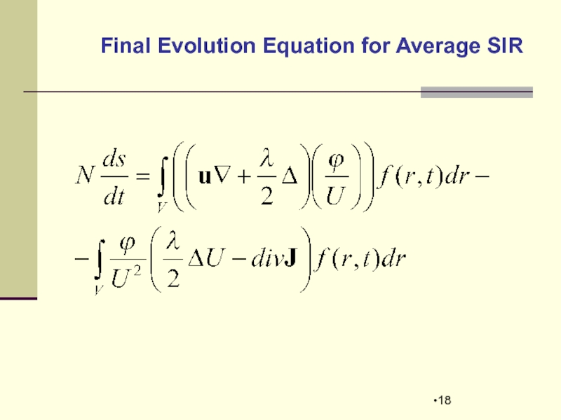
Слайд 15SIR value in a continuous media
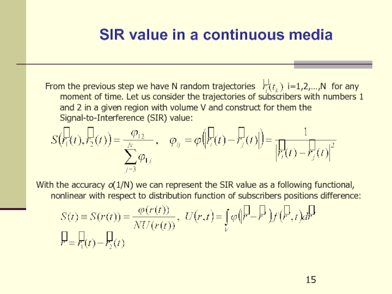
From the previous step we have
With the accuracy o(1/N) we can represent the SIR value as a following functional, nonlinear with respect to distribution function of subscribers positions difference:
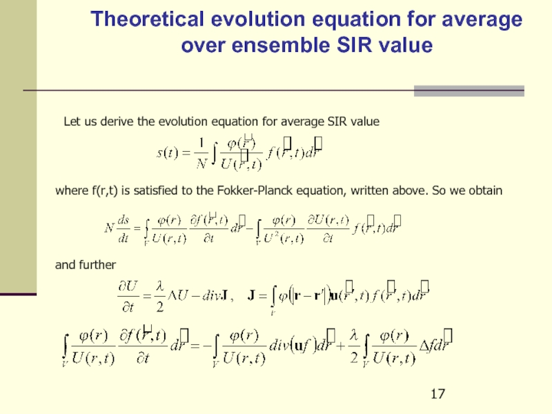
Слайд 17Let us derive the evolution equation for average SIR value
where f(r,t)
and further
Theoretical evolution equation for average over ensemble SIR value
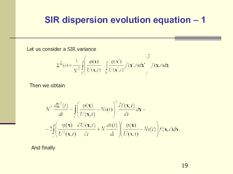
Слайд 19SIR dispersion evolution equation – 1
Let us consider a SIR
Then we obtain
And finally
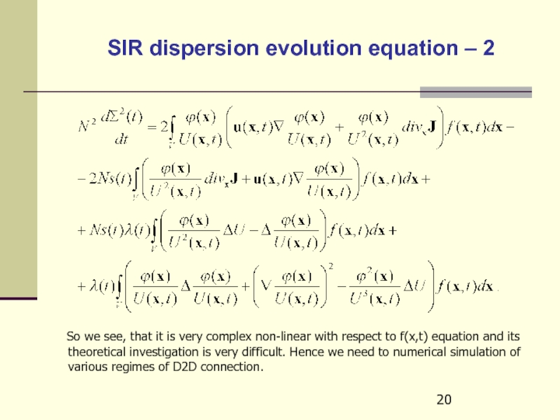
Слайд 20SIR dispersion evolution equation – 2
So we
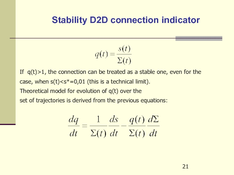
Слайд 21Stability D2D connection indicator
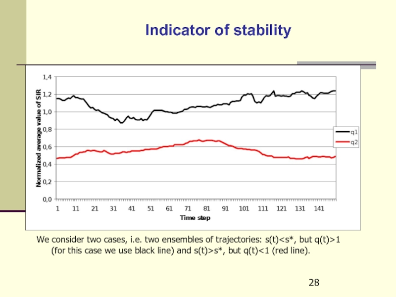
If q(t)>1, the connection can be treated
case, when s(t)
set of trajectories is derived from the previous equations:
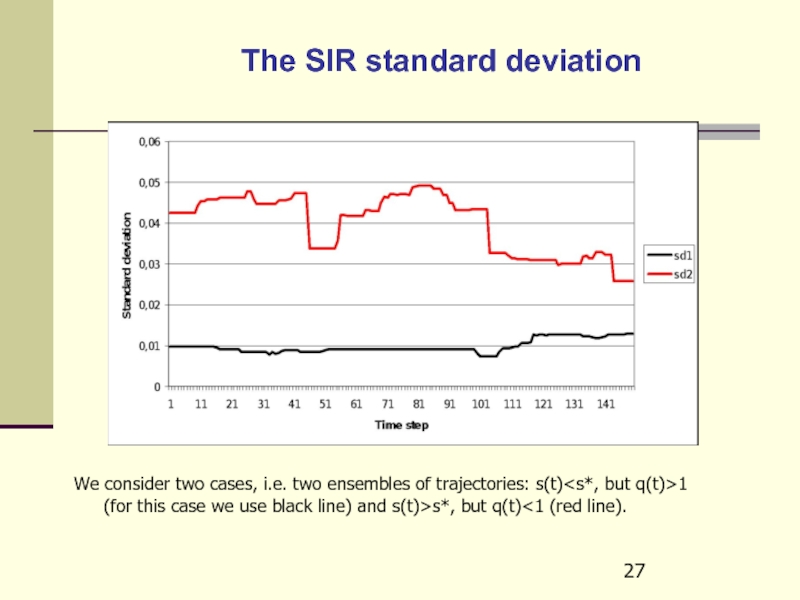
Слайд 27The SIR standard deviation
We consider two cases, i.e. two ensembles
Слайд 28Indicator of stability
We consider two cases, i.e. two ensembles of
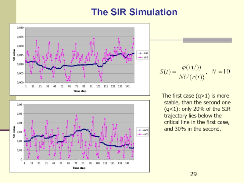
Слайд 29The SIR Simulation
The first case (q>1) is more
Слайд 31
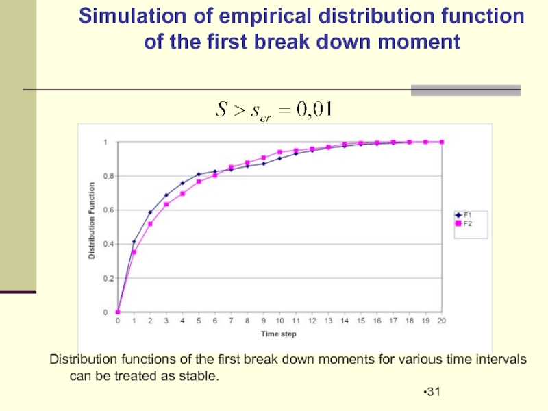
Simulation of empirical distribution function of the first break down moment
Distribution functions of the first break down moments for various time intervals can be treated as stable.
Слайд 32
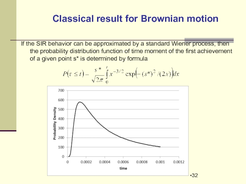
Classical result for Brownian motion
If the SIR behavior can be
Слайд 33
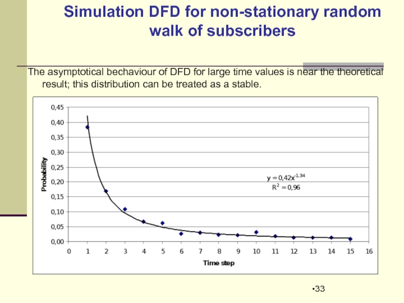
Simulation DFD for non-stationary random walk of subscribers
The asymptotical bechaviour
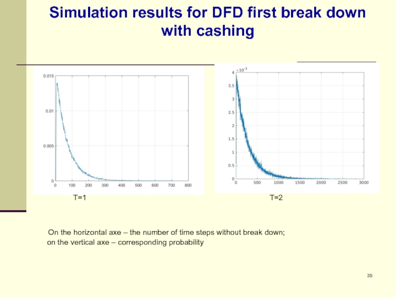
Слайд 35Simulation results for DFD first break down with cashing
T=1
On the horizontal axe – the number of time steps without break down;
on the vertical axe – corresponding probability
Слайд 38Conclusions
Numerical simulation the SIR trajectory for an arbitrary pare of abonents,
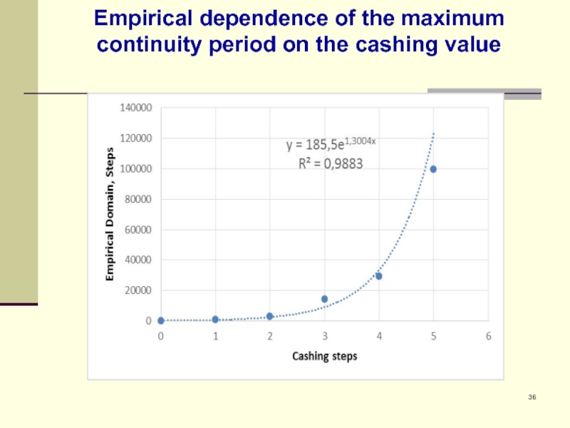
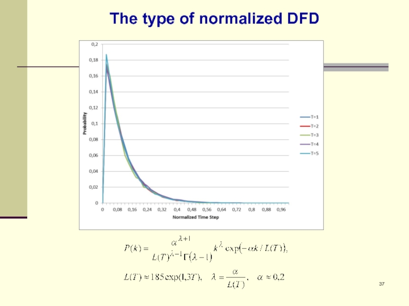
DFD of break down moments without cashing has a power-law tail; DFD with cashing can be treated as a gamma-distribution. DFD Domain increases exponentially with cashing period. DFD’s for various cashing periods can be converted to the same unique distribution.
We presents here some abstract situation, but it can be easily recalculated to the practical problem. The main result is that the cashing period, needed for continuity of wireless connection, is rather short du to exponential decreasing of break down probability.
Слайд 39
The main references
1. Orlov Yu.N., Fedorov S.L. 2016. Modelirovanie raspredelenij funkcionalov
URL: http://library.keldysh.ru/preprint.asp?id=2016-101
2. Yu. Gaidamaka, Yu. Orlov, S. Fedorov, A. Samuylov, D. Molchanov. 2016. Simulation of Devices Mobility to Estimate Wireless Channel Quality Metrics in 5G Network. Proc. ICNAAM, September 19-25, Rhodes, Greece.
3. Fedorov S.L., Orlov Yu.N. 2016. Metody chislennogo modelirovaniya processov nestatsionarnogo sluchajnogo bluzhdaniya (in Russian). – Moscow: MIPT.
4. Orlov Yu.N., Fedorov S.L. 2016. Generation of non-stationary time-series trajectories on the basis of Fokker-Planck equation (in Russian). Trudy MIPT, 8, No. 2, 126-133.
5. Orlov Yu.N., Fedorov S.L. 2016. Modelirovanie ansamblya nestacionarnyh traektorij s pomoshch'yu uravneniya Fokkera-Planka (in Russian). Zhurnal Srednevolzhskogo matematicheskogo obshchestva, No1.
6. Orlov Yu.N., Fedorov S.L. 2017. Modelirovanie ansamblia nestatsionarnyh sluchainyh traektorij s ispolzovaniem uravnenija Fokkera-Planka (in russian) // Matematicheskoe modelirovanie, V. 29. № 5. P. 61-72.
7. Orlov Yu.N., Fedorov S.L., Samoulov A.K., Gaidamaka Yu.V., Molchanov D.A. Simulation of Devices Mobility to Estimate Wireless Channel Quality Metrics in 5G Network // AIP Conference Proceedings, 2017. V. 1863, 090005.
