- Главная
- Разное
- Дизайн
- Бизнес и предпринимательство
- Аналитика
- Образование
- Развлечения
- Красота и здоровье
- Финансы
- Государство
- Путешествия
- Спорт
- Недвижимость
- Армия
- Графика
- Культурология
- Еда и кулинария
- Лингвистика
- Английский язык
- Астрономия
- Алгебра
- Биология
- География
- Детские презентации
- Информатика
- История
- Литература
- Маркетинг
- Математика
- Медицина
- Менеджмент
- Музыка
- МХК
- Немецкий язык
- ОБЖ
- Обществознание
- Окружающий мир
- Педагогика
- Русский язык
- Технология
- Физика
- Философия
- Химия
- Шаблоны, картинки для презентаций
- Экология
- Экономика
- Юриспруденция
Macroeconomics Productivity Output Employment. (Lecture 5) презентация
Содержание
- 1. Macroeconomics Productivity Output Employment. (Lecture 5)
- 2. How much does the economy produce? The
- 3. Factors affecting productivity Technology Inputs Labor
- 4. The production function The quantity of inputs
- 5. Empirical example: US production function Studies show
- 6. Calculating “A”
- 7. Shape of the production function We can
- 8. Shape of the production function
- 9. Shape of the production function: Properties The
- 10. Effect of increasing 1000 units of capital
- 11. Marginal productivity The previous example shows that
- 12. Formal Definitions of Marginal Productivity Marginal Productivity
- 13. Changes in the production function The production
- 14. Demand for labor In contrast to the
- 15. Determination of the demand for labor Demand
- 16. Determination of demand for labor To maximize
- 17. Determination of labor demand w* N*
- 18. Factors that shift labor demand curve Changes
- 19. Shift of the labor demand curve A
- 20. Supply of labor We have seen that
- 21. Labor supply curve Labor supply curve looks
- 22. Factors that shift the labor supply curve Left Left Right Right
- 23. Labor market equilibrium w* MPN
- 24. When profit maximizing wage is higher than
- 25. Effects of adverse supply shock W2 N2
- 26. What if all workers are not alike?
- 27. Unemployment: the untold story of full-employment Full-employment
Слайд 2How much does the economy produce?
The quantity that an economy will
The quantity of inputs utilized in the production process and
The PRODUCTIVITY of the inputs
An economy’s productivity is basic to determining living standards.
In this lecture we shall see how productivity affects people’s incomes by helping to determine how many workers are employed and how much they receive.
Among all the inputs for production, labor is usually considered the most important input.
Therefore, first we shall study the factors that determine demand and supply of labor and then the forces that bring the labor market into equilibrium.
Equilibrium in the labor market determines wages and employment; and the level of employment together with other inputs and the level of productivity determines how much output en economy produces.
Слайд 3Factors affecting productivity
Technology
Inputs
Labor
Capital
Land
Raw materials
Machinery
Power
Time period
Слайд 4The production function
The quantity of inputs does not completely determine the
How effectively the factors of production are used is also important.
The effectiveness with which factors of production are used may be expressed by a relationship called the production function.
Mathematically, we express production function as-
Y = A f(K, N, L, …)
Where, Y stands for output, A - number that indicated productivity, K - capital, N – number of labor employed, L - land. Other factors could be, machinery, energy, building etc.
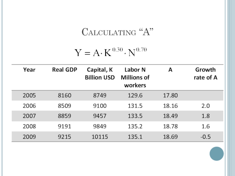
The symbol “A” in the equation above captures the overall effectiveness of the factors of production. We call A the “total factor productivity”
Слайд 5Empirical example: US production function
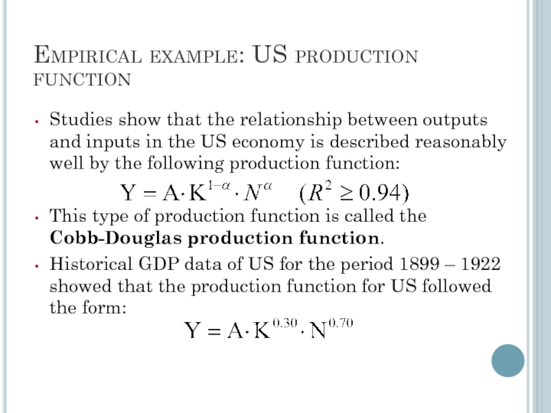
Studies show that the relationship between outputs
This type of production function is called the Cobb-Douglas production function.
Historical GDP data of US for the period 1899 – 1922 showed that the production function for US followed the form:
Слайд 7Shape of the production function
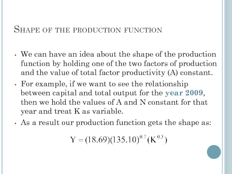
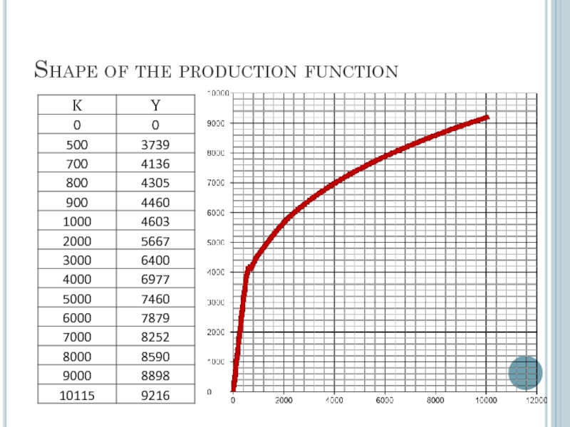
We can have an idea about the
For example, if we want to see the relationship between capital and total output for the year 2009, then we hold the values of A and N constant for that year and treat K as variable.
As a result our production function gets the shape as:
Слайд 9Shape of the production function: Properties
The production function slopes upward from
The slope of the production function becomes flatter from left to right: this means that although more capital always leads to more output, it does so at a decreasing rate.
Слайд 10Effect of increasing 1000 units of capital each time
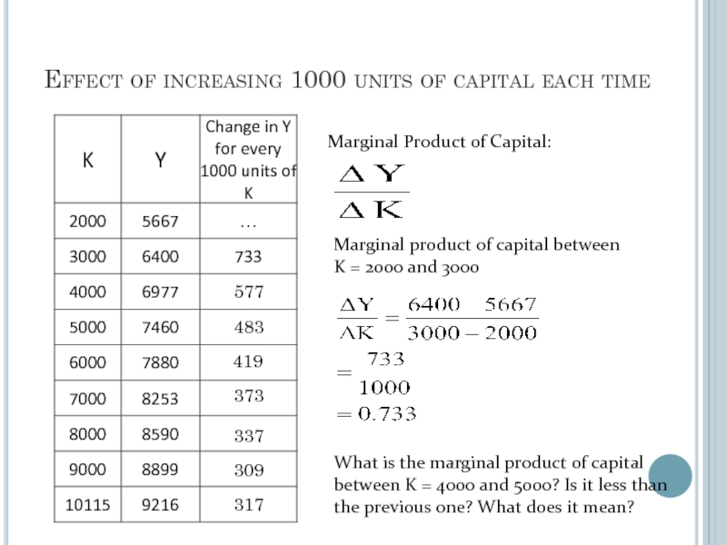
Marginal Product of
Marginal product of capital between
K = 2000 and 3000
What is the marginal product of capital between K = 4000 and 5000? Is it less than the previous one? What does it mean?
577
483
419
373
337
309
317
Слайд 11Marginal productivity
The previous example shows that marginal productivity is falling as
Generally, when amount of labor is high compared to the amount of capital, marginal productivity of capital is high. Alternatively, when amount of labor is low compared to the amount of capital, marginal productivity of labor is high
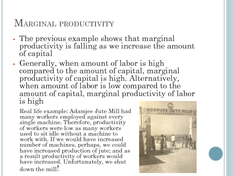
Real life example: Adamjee Jute Mill had many workers employed against every single machine. Therefore, productivity of workers were low as many workers used to sit idle without a machine to work with. If we would have increased number of machines, perhaps, we could have increased production of jute; and as a result productivity of workers would have increased. Unfortunately, we shut down the mill!
Слайд 12Formal Definitions of Marginal Productivity
Marginal Productivity of Capital: means additional output
Marginal Productivity of Labor: means additional output produced by each additional unit of labor.
Because of diminishing marginal productivity for both labor and capital the slope of production function becomes flatter from left to right.
If the marginal productivity were increasing, slope of the production function would become steeper from left to right.
If the marginal productivity were constant, the slope would be constant and the shape of the curve of production function would be a straight line.
Слайд 13Changes in the production function
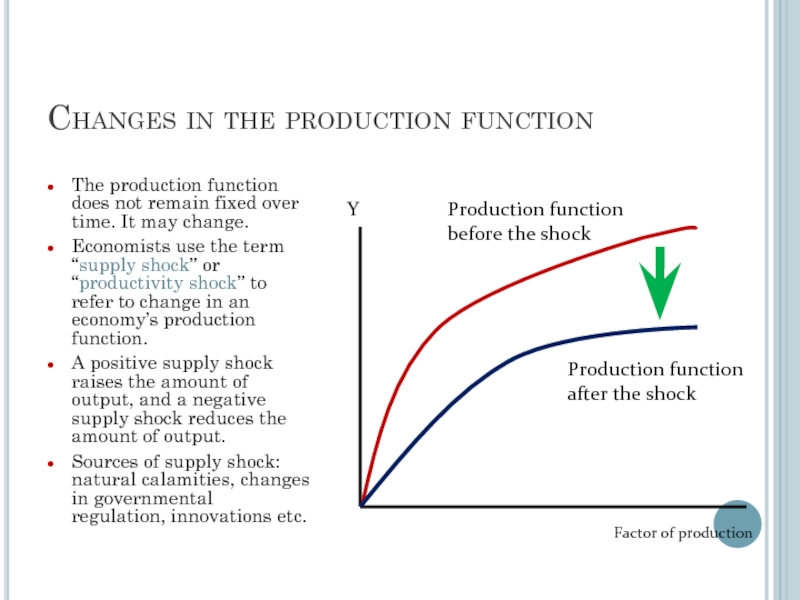
The production function does not remain fixed
Economists use the term “supply shock” or “productivity shock” to refer to change in an economy’s production function.
A positive supply shock raises the amount of output, and a negative supply shock reduces the amount of output.
Sources of supply shock: natural calamities, changes in governmental regulation, innovations etc.
Production function before the shock
Production function after the shock
Y
Factor of production
Слайд 14Demand for labor
In contrast to the amount of capital, the amount
Thus, year-to-year changes in production can be traced to the changes in employment.
Demand for labor determines the level of employment.
For this reason, understanding demand for labor is important.
To understand demand for labor we shall make the following assumptions to keep things simple:
Workers are alike
Firms have to pay competitive wage to hire workers
Firms objective is to maximize profit
Слайд 15Determination of the demand for labor
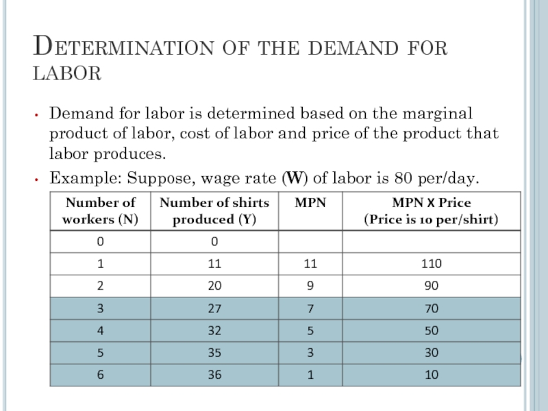
Demand for labor is determined based
Example: Suppose, wage rate (W) of labor is 80 per/day.
Слайд 16Determination of demand for labor
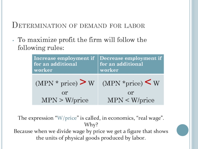
To maximize profit the firm will follow
The expression “W/price” is called, in economics, “real wage”. Why?
Because when we divide wage by price we get a figure that shows the units of physical goods produced by labor.
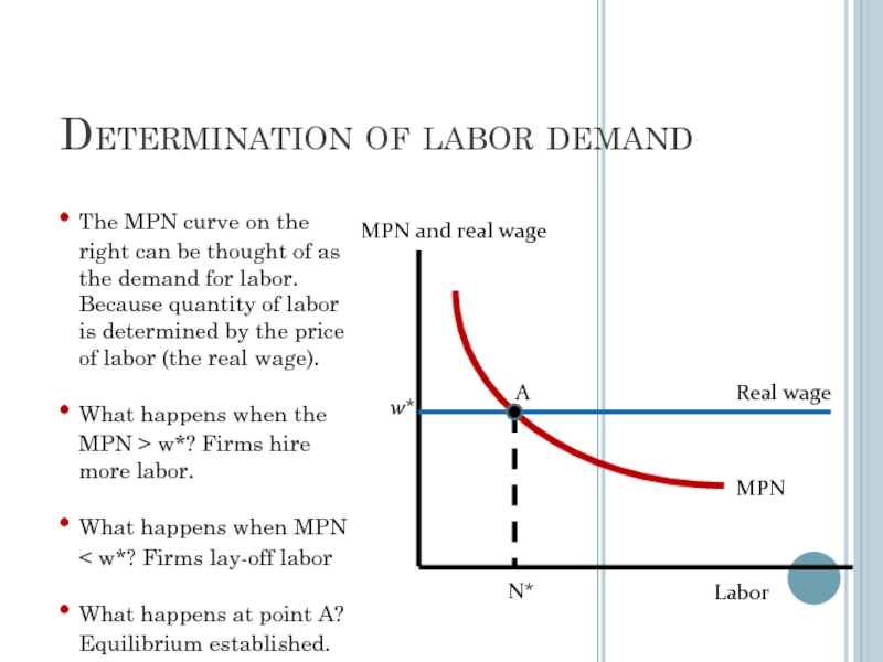
Слайд 17Determination of labor demand
w*
N*
MPN and real wage
Labor
MPN
Real wage
The MPN curve on
What happens when the MPN > w*? Firms hire more labor.
What happens when MPN < w*? Firms lay-off labor
What happens at point A? Equilibrium established.
A
Слайд 18Factors that shift labor demand curve
Changes in the wage do not
Factors that shift labor demand curve would be something that will change the demand for labor at any given wage.
A beneficial shock will shift the labor demand curve to the right.
An adverse shock will shift the labor demand curve to the left.
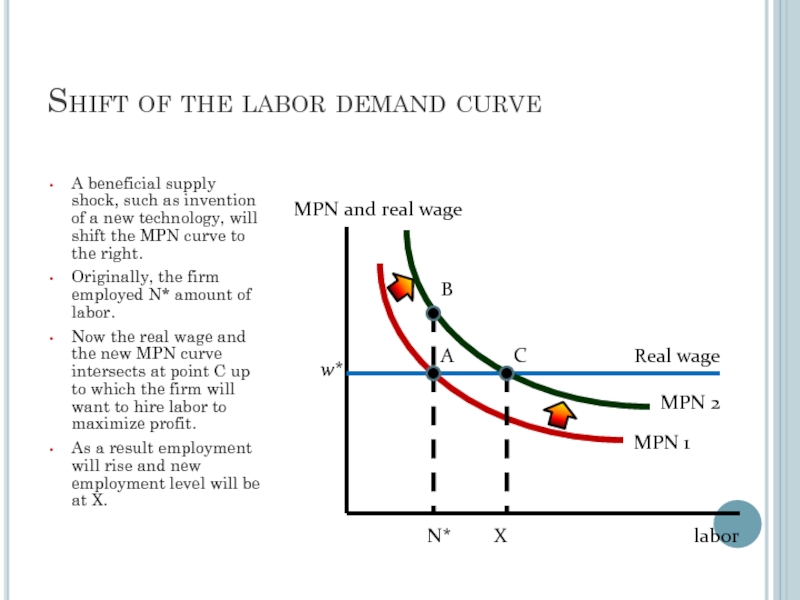
Слайд 19Shift of the labor demand curve
A beneficial supply shock, such as
Originally, the firm employed N* amount of labor.
Now the real wage and the new MPN curve intersects at point C up to which the firm will want to hire labor to maximize profit.
As a result employment will rise and new employment level will be at X.
w*
N*
MPN and real wage
labor
MPN 1
Real wage
A
C
MPN 2
B
X
Слайд 20Supply of labor
We have seen that firm’s demand for labor depend
However, supply of labor depends on workers’ personal choice to work.
Personal choice about being a part of the labor force generally depends on the following two factors:
Income-leisure trade-off
Real wage
Слайд 21Labor supply curve
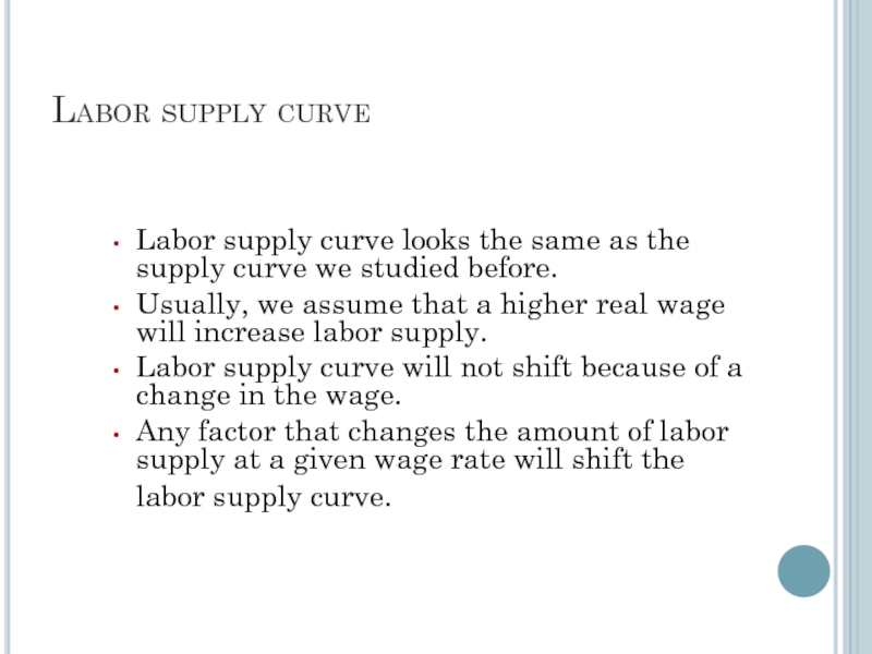
Labor supply curve looks the same as the supply
Usually, we assume that a higher real wage will increase labor supply.
Labor supply curve will not shift because of a change in the wage.
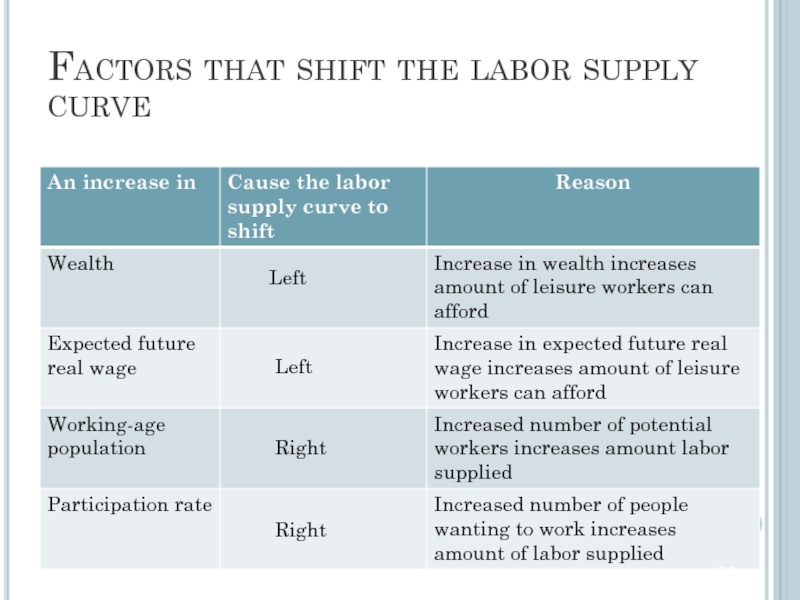
Any factor that changes the amount of labor supply at a given wage rate will shift the labor supply curve.
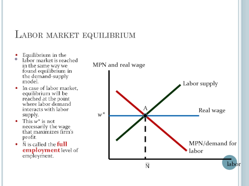
Слайд 23Labor market equilibrium
w*
MPN and real wage
labor
MPN/demand for labor
Real wage
A
Labor supply
Слайд 24When profit maximizing wage is higher than equilibrium wage
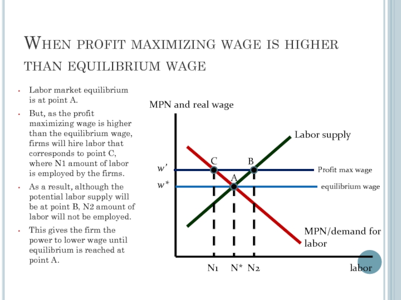
Labor market equilibrium
But, as the profit maximizing wage is higher than the equilibrium wage, firms will hire labor that corresponds to point C, where N1 amount of labor is employed by the firms.
As a result, although the potential labor supply will be at point B, N2 amount of labor will not be employed.
This gives the firm the power to lower wage until equilibrium is reached at point A.
w*
N*
MPN and real wage
labor
MPN/demand for labor
equilibrium wage
A
Profit max wage
w’
C
B
N2
N1
Labor supply
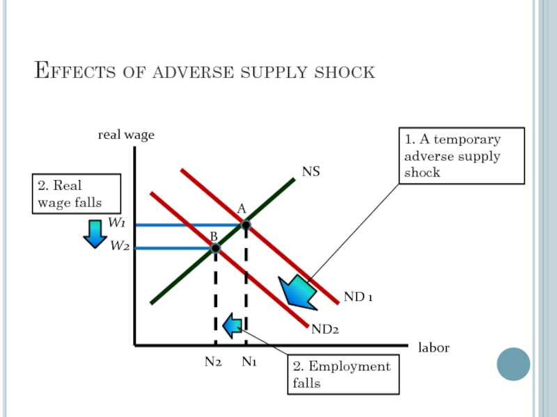
Слайд 25Effects of adverse supply shock
W2
N2
real wage
labor
ND 1
B
N1
ND2
A
W1
NS
1. A temporary adverse supply
2. Employment falls
2. Real wage falls
Слайд 26What if all workers are not alike?
We assumed that all workers
However, if workers have different skill level then supply shocks will not affect all workers in the same way.
Example: if a production process introduces computer based production, then workers who can operate computers will cope with the new process quickly. On the other hand, workers who cannot operate computers will find it difficult to cope with the process. This will create difference in the marginal productivity level of these two groups of workers. Most likely, the workers who can use computers will get higher wage at cost of those who cannot.
Therefore, whether a shock will be considered beneficial or adverse depends on the skill/education level of the workers.
Слайд 27Unemployment: the untold story of full-employment
Full-employment level implies that all the
All workers in real life do not find jobs even if they want to. When workers are unemployed for a long time the sum of all such workers constitute “structural unemployment”.
If workers are unemployed for a brief period (for example: the brief period in which they search for a suitable job) we call it “frictional unemployment”.
The rate of unemployment that prevails when output and unemployment rate the full-employment level, we call it natural rate of unemployment.
The difference between actual unemployment rate and natural unemployment rate is called cyclical unemployment.
If workers are not willing to work, this will not constitute unemployment. We shall consider these workers as out of work force.
