- Главная
- Разное
- Дизайн
- Бизнес и предпринимательство
- Аналитика
- Образование
- Развлечения
- Красота и здоровье
- Финансы
- Государство
- Путешествия
- Спорт
- Недвижимость
- Армия
- Графика
- Культурология
- Еда и кулинария
- Лингвистика
- Английский язык
- Астрономия
- Алгебра
- Биология
- География
- Детские презентации
- Информатика
- История
- Литература
- Маркетинг
- Математика
- Медицина
- Менеджмент
- Музыка
- МХК
- Немецкий язык
- ОБЖ
- Обществознание
- Окружающий мир
- Педагогика
- Русский язык
- Технология
- Физика
- Философия
- Химия
- Шаблоны, картинки для презентаций
- Экология
- Экономика
- Юриспруденция
Macroeconomics. Introduction презентация
Содержание
- 1. Macroeconomics. Introduction
- 2. Introduction Structure of course Chapter 1
- 3. Introduction Structure of course Chapter 5
- 4. Introduction Structure of course Chapter 7
- 5. Introduction Structure of course Chapter 9
- 6. Introduction Definition “Macroeconomics was born as
- 7. Introduction Definition Since then, economic
- 8. Introduction Definition Since then, economic
- 9. Introduction Relationships between two sub-
- 10. Introduction An overview of the macroeconomic
- 11. Introduction An overview of the macroeconomic theories
- 12. Introduction An overview of the macroeconomic theories
- 13. Introduction An overview of the macroeconomic theories
- 14. Introduction An overview of the macroeconomic theories
- 15. Introduction The Empirical Aspects of the Macro-economics
- 16. Introduction The Empirical Aspects of the Macro-economics
- 17. Introduction The Empirical Aspects of the Macro-economics
- 18. Introduction The Empirical Aspects of the Macro-economics Macroeconomic subjects
- 19. Introduction The Empirical Aspects of the Macro-economics OUTPUT=INCOME=EXPENDITURE
- 20. Introduction The measurement of macroeconomic facts Economic
- 21. Introduction The measurement of macroeconomic facts Measurement
- 22. Introduction The measurement of macroeconomic facts Measurement
- 23. Introduction The measurement of macroeconomic facts Measurement
- 24. Introduction The measurement of macroeconomic facts Measurement
- 25. Introduction Methods and Assumptions of Macro-economic
- 26. Introduction Methods and Assumptions of Macro-economic
- 27. The determination of Output, Income, Expenditure and
- 28. The determination of Output, Income, Expenditure and
- 29. The determination of Output, Income, Expenditure and
- 30. The determination of Output, Income, Expenditure and
- 31. The determination of Output, Income, Expenditure and
- 32. The determination of Output, Income, Expenditure and
- 33. The determination of Output, Income, Expenditure and
- 34. The determination of Output, Income, Expenditure and
- 35. The determination of Output, Income, Expenditure and
- 36. The determination of Output, Income, Expenditure and
- 37. The determination of Output, Income, Expenditure and
- 38. The determination of Output, Income, Expenditure and
- 39. The determination of Output, Income, Expenditure and
- 40. The determination of Output, Income, Expenditure and
- 41. The determination of Output, Income, Expenditure and
- 42. The determination of Output, Income, Expenditure and
- 43. The determination of Output, Income, Expenditure and
- 44. The determination of Output, Income, Expenditure and
- 45. The determination of Output, Income, Expenditure and
- 46. The determination of Output, Income, Expenditure and
- 47. The determination of Output, Income, Expenditure and
- 48. The determination of Output, Income, Expenditure and
- 49. The determination of Output, Income, Expenditure and
- 50. The determination of Output, Income, Expenditure and
- 51. Money, prices and interest rates What is
- 52. Money, prices and interest rates Money is
- 53. Money, prices and interest rates Agents will
- 54. Money, prices and interest rates The Quantity
- 55. Money, prices and interest rates The Quantity
- 56. Money, prices and interest Rates The Interest
- 57. Money, prices and interest Rates The Interest
- 58. Money, prices and interest Rates The Interest
- 59. Money, prices and interest Rates Interest rate
- 60. Money, prices and interest Rates The money
- 61. Money, prices and interest rates The money
- 62. Money, prices and interest rates The Problems
- 63. Money, prices and interest rates The Problems
- 64. Labour market, employment, unemployment Labour demand
- 65. Labour market, employment, unemployment The labour force
- 66. Labour market, employment, unemployment The labour force
- 67. Labour market, employment, unemployment The labour force
- 68. Labour market, employment, unemployment N=E+U+I
- 69. Labour market, employment, unemployment Share of long
- 70. Labour market, employment, unemployment The flow of
- 71. The Long-Run Rate of Unemployment
- 72. The Long-Run Rate of Unemployment
- 73. The Long-Run Rate of Unemployment Natural rate of unemployment=long-run rate of unemployment A=P
- 74. Economic fluctuations The economy is
- 75. Economic fluctuations Acceleration phases (economic boom) Contraction phase (economic recession)
- 76. Economic fluctuations Changes in output
- 77. Economic fluctuations Changes in output
- 78. Economic fluctuations Changes in output
- 79. Economic fluctuations Aggregate demand and
- 80. Economic fluctuations Aggregate demand and
- 81. Economic fluctuations Aggregate demand and
- 82. Economic fluctuations Aggregate demand and
- 83. Economic fluctuations Aggregate demand and
- 84. Economic fluctuations Aggregate demand and
- 85. Economic fluctuations Aggregate demand and
- 86. Economic fluctuations Aggregate demand and
- 87. Economic fluctuations External shock –an event
- 88. The Keynesian Model of Short-Run Equilibrium Model
- 89. The Keynesian Model of Short-Run Equilibrium Model
- 90. The Keynesian Model of Short-Run Equilibrium Model
- 91. The Keynesian Model of Short-Run Equilibrium Model
- 92. The Keynesian Model of Short-Run Equilibrium Model
- 93. The Keynesian Model of Short-Run Equilibrium Model
- 94. The Keynesian Model of Short-Run Equilibrium Model
- 95. The Keynesian Model of Short-Run Equilibrium Model
- 96. The Keynesian Model of Short-Run Equilibrium Model
- 97. The Keynesian Model of Short-Run Equilibrium Model
- 98. The Keynesian Model of Short-Run Equilibrium Model
- 99. The Keynesian Model of Short-Run Equilibrium Model
- 100. The Keynesian Model of Short-Run Equilibrium Model
- 101. Aggregate Supply LRAS –level of output is
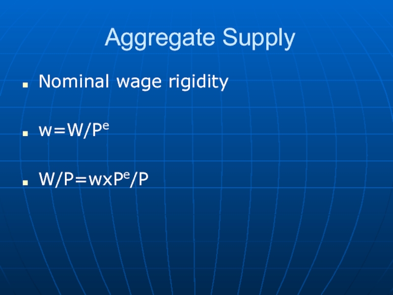
- 102. Aggregate Supply Nominal wage rigidity w=W/Pe W/P=wxPe/P
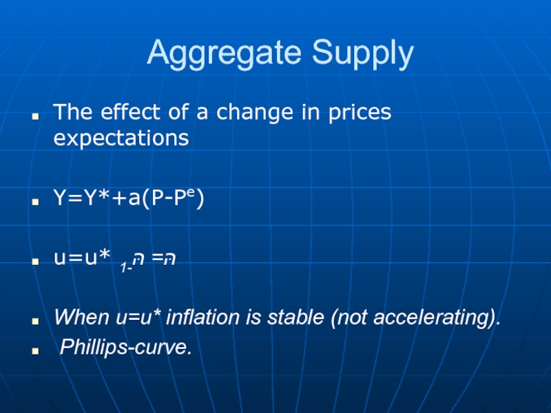
- 103. Aggregate Supply The effect of a change
Слайд 2Introduction
Structure of course
Chapter 1 The date and methods of macroeconomics
Chapter
Слайд 3Introduction
Structure of course
Chapter 5 The Determination of Output, Income, Expenditure and
Chapter 6 Money, Prices and the Interest Rate
Слайд 4Introduction
Structure of course
Chapter 7 Labour Market, Employment, Unemployment
Chapter 8 Economic
Слайд 5Introduction
Structure of course
Chapter 9 The Keynsian Model of
Short-Run
Chapter 10 Aggregate Supply
Слайд 6Introduction
Definition
“Macroeconomics was born as distinct in the 1940, as part
(R. Lucas)
Слайд 7Introduction
Definition
Since then, economic science is divided into two fields
Microeconomics, which develops the theories of individual behaviors: theories of producer, consumer, etc.
Слайд 8Introduction
Definition
Since then, economic science is divided into two fields
Macroeconomics, which develops the theories of collective behaviors
The main goal of macroeconomics is to explain and predict the evolution of different economic variables, such as output, employment, money supply, interest rates, prices, exchange rates, external balance, public budget deficit, public debt
Слайд 9Introduction
Relationships between two sub-
disciplines
Examples
- the level of public deficit (macro) can get people to change their saving behaviours (micro)
Слайд 10Introduction
An overview of the macroeconomic theories
Two main theories:
- Keynesian theory – “ sticky prices macroeconomics”
Слайд 11Introduction
An overview of the macroeconomic theories
Classical theory- economic policies are not
Слайд 12Introduction
An overview of the macroeconomic theories
Keynesian theory – economic policies are
Слайд 13Introduction
An overview of the macroeconomic theories
Classical theory-
Hypothesis of flexible prices, macroeconomic
Слайд 14Introduction
An overview of the macroeconomic theories
Keynsian theory helps to explain the
Слайд 15Introduction
The Empirical Aspects of the Macro-economics
The macro circuit means a non-theoretical
Three macroeconomic aggre-gates: global output, global income, global expenditure.
Слайд 16Introduction
The Empirical Aspects of the Macro-economics
The output is the value, expressed
Income means the monetary value of resources received by agents
Слайд 17Introduction
The Empirical Aspects of the Macro-economics
Expenditure means the money value of
Слайд 20Introduction
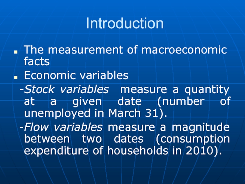
The measurement of macroeconomic facts
Economic variables
-Stock variables measure a quantity
-Flow variables measure a magnitude between two dates (consumption expenditure of households in 2010).
Слайд 21Introduction
The measurement of macroeconomic facts
Measurement of output
The nominal output
- QV ALt = ∑qit pit
Слайд 22Introduction
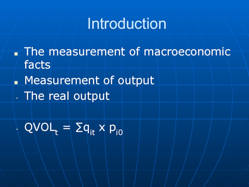
The measurement of macroeconomic facts
Measurement of output
The real output
QVOLt = ∑qit
Слайд 23Introduction
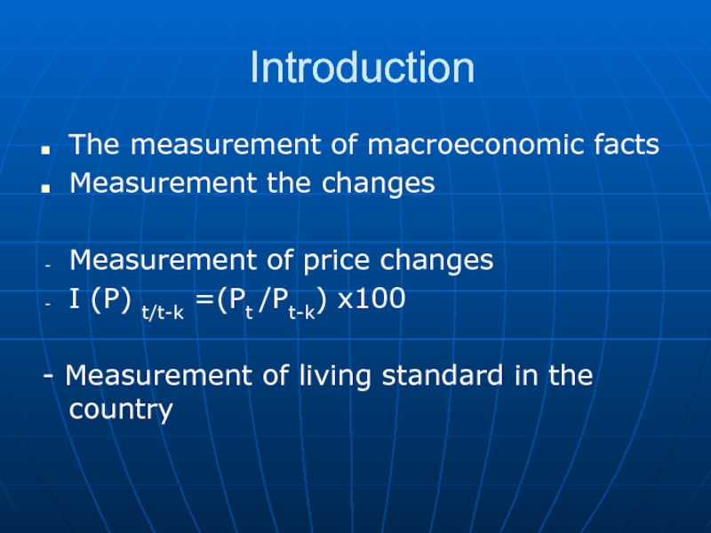
The measurement of macroeconomic facts
Measurement the changes
Measurement of price changes
I
- Measurement of living standard in the country
Слайд 24Introduction
The measurement of macroeconomic facts
Measurement the productivity
Y/H hourly labour productivity
Слайд 25Introduction
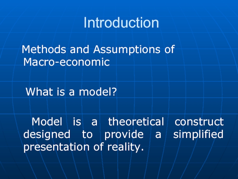
Methods and Assumptions of Macro-economic
What is a
Model is a theoretical construct designed to provide a simplified presentation of reality.
Слайд 26Introduction
Methods and Assumptions of Macro-economic
What is a
Example- a model of economic equilibrium
Слайд 27The determination of Output, Income, Expenditure and a model of Real
The production function and aggregate supply
Y=F (K,L)
Output will depend on amounts of factor use but also on returns to scale
Слайд 28The determination of Output, Income, Expenditure and a model of Real
The production function and aggregate supply
F (λK,λL)= λzY
z=1 constant returns to scale
Z<1 decreasing returns to scale
Z>1 increasing returns to scale
Слайд 29The determination of Output, Income, Expenditure and a model of Real
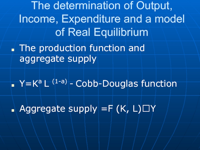
The production function and aggregate supply
Y=Ka L (1-a) - Cobb-Douglas function
Aggregate supply =F (K, L)?Y
Слайд 30The determination of Output, Income, Expenditure and a model of Real
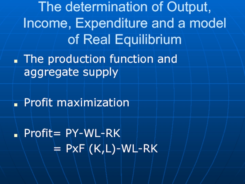
The production function and aggregate supply
Profit maximization
Profit= PY-WL-RK
= PxF (K,L)-WL-RK
Слайд 31The determination of Output, Income, Expenditure and a model of Real
The production function and aggregate supply
MPL marginal product of labour
MPL=F(K, L+1)-F (K,L)
Слайд 32The determination of Output, Income, Expenditure and a model of Real
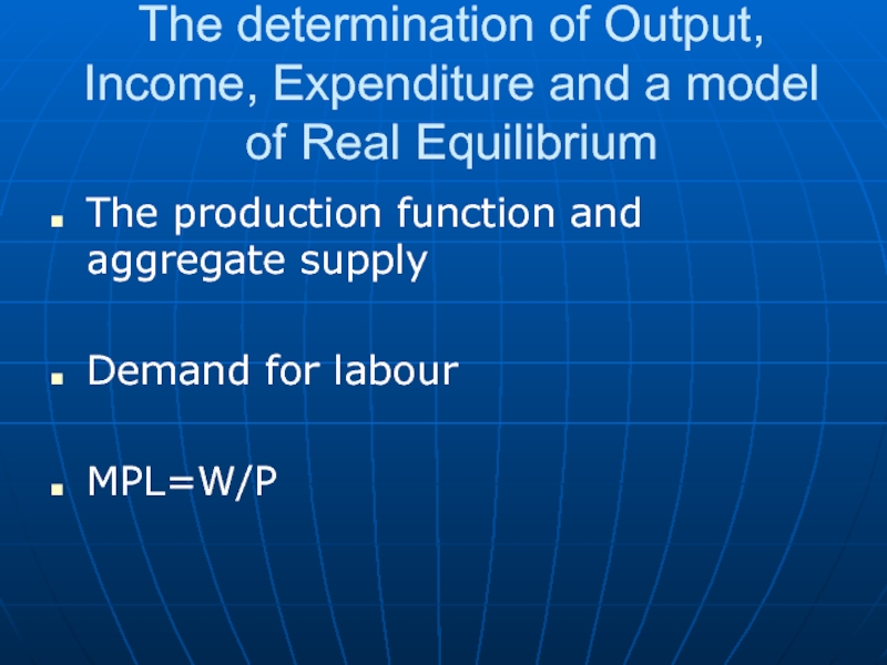
The production function and aggregate supply
Demand for labour
MPL=W/P
Слайд 33The determination of Output, Income, Expenditure and a model of Real
The production function and aggregate supply
Demand for capital
MPK=F(K+1,L)-F(K,L)
MPK=R/P
Слайд 34The determination of Output, Income, Expenditure and a model of Real
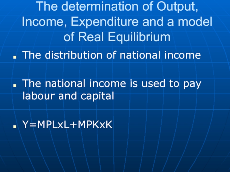
The distribution of national income
The national income is used to pay labour and capital
Y=MPLxL+MPKxK
Слайд 35The determination of Output, Income, Expenditure and a model of Real
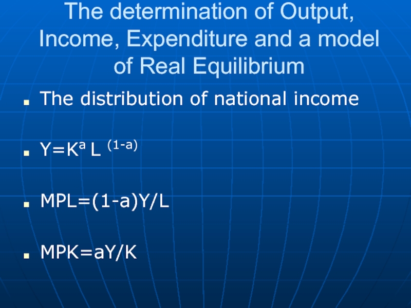
The distribution of national income
Y=Ka L (1-a)
MPL=(1-a)Y/L
MPK=aY/K
Слайд 36The determination of Output, Income, Expenditure and a model of Real
The distribution of national income
Y=Ka L (1-a)
MPL=(1-a)Y/L
MPK=aY/K
Слайд 37The determination of Output, Income, Expenditure and a model of Real
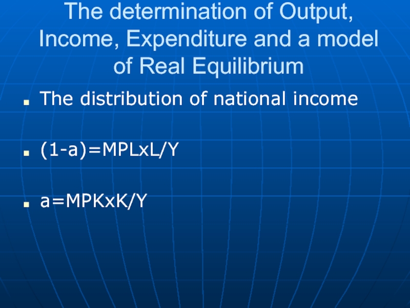
The distribution of national income
(1-a)=MPLxL/Y
a=MPKxK/Y
Слайд 38The determination of Output, Income, Expenditure and a model of Real
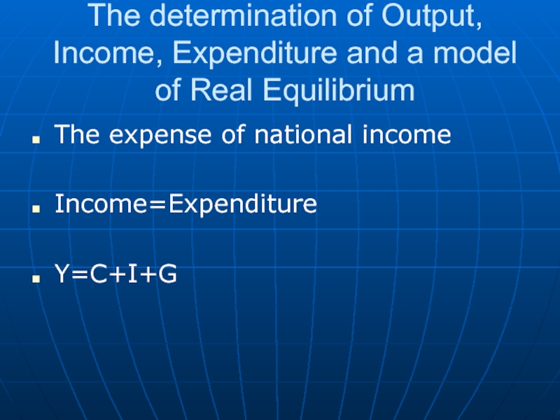
The expense of national income
Income=Expenditure
Y=C+I+G
Слайд 39The determination of Output, Income, Expenditure and a model of Real
The expense of national income
The consumption function
Classical economists consider that savings is determined by the rate of interest.
Слайд 40The determination of Output, Income, Expenditure and a model of Real
The expense of national income
The consumption function
Keynesian economists consider that most influent variable for consumption is level of income. (Psychological fundamental law).
Слайд 41The determination of Output, Income, Expenditure and a model of Real
The expense of national income
The consumption function
In keynesian economics
MPC=∆C/ ∆(Y-T) marginal propensity to consume
Слайд 42The determination of Output, Income, Expenditure and a model of Real
The expense of national income
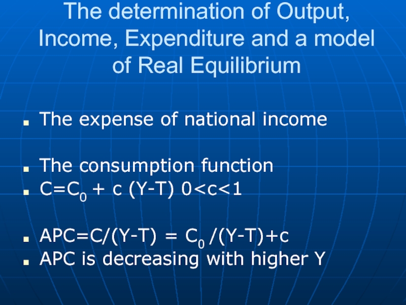
The consumption function
C=C0 + c (Y-T) 0
APC=C/(Y-T) = C0 /(Y-T)+c
APC is decreasing with higher Y
Слайд 43The determination of Output, Income, Expenditure and a model of Real
The expense of national income
The investment function
The decision to invest at the micro level
The decision rule
For a given project the investment will be achieved only if r>r*
Слайд 44The determination of Output, Income, Expenditure and a model of Real
The expense of national income
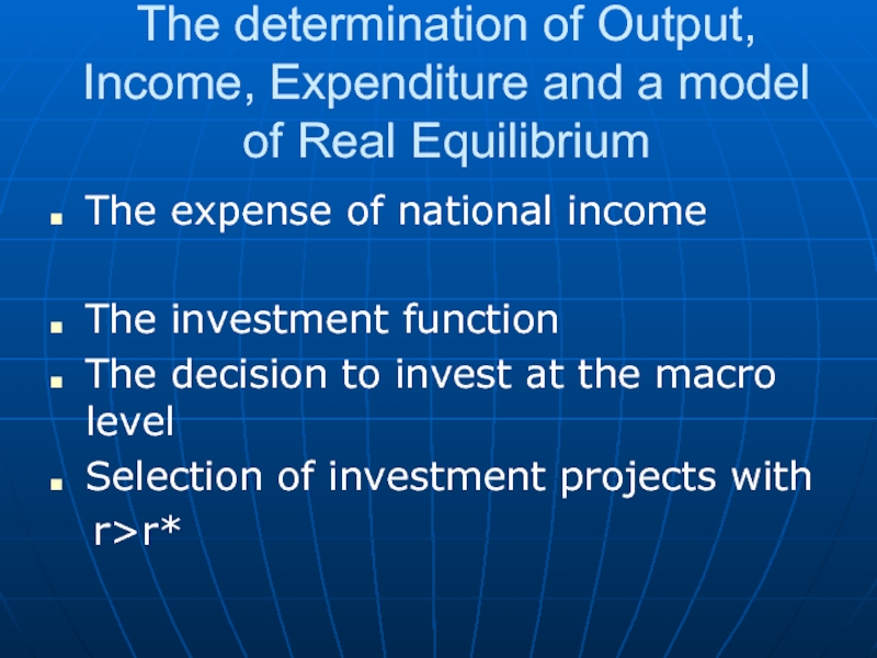
The investment function
The decision to invest at the macro level
Selection of investment projects with
r>r*
Слайд 45The determination of Output, Income, Expenditure and a model of Real
The expense of national income
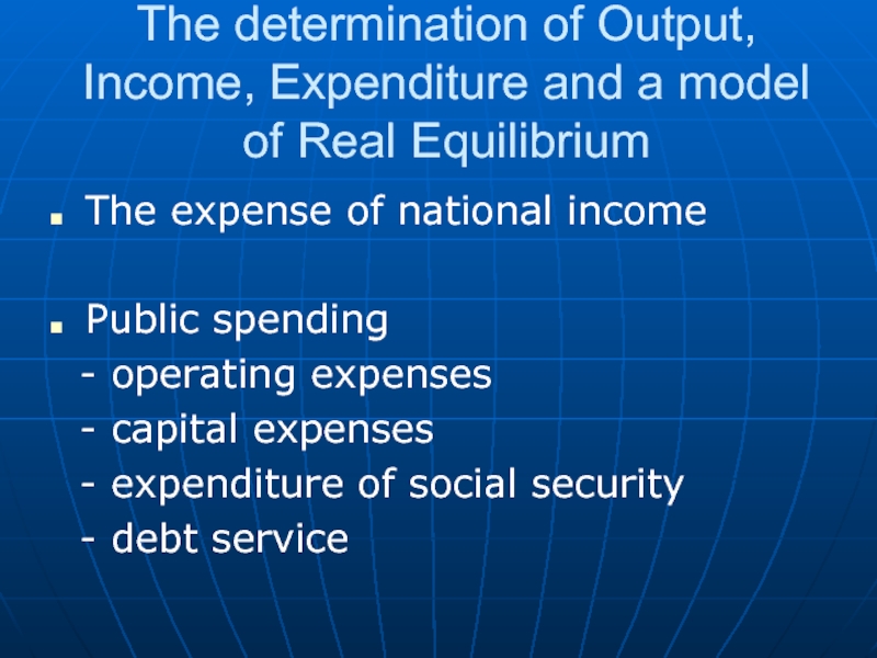
Public spending
- operating expenses
- capital expenses
- expenditure of social security
- debt service
Слайд 46The determination of Output, Income, Expenditure and a model of Real
The expense of national income
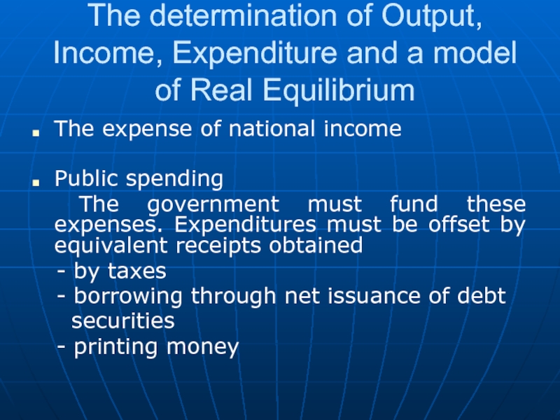
Public spending
The government must fund these expenses. Expenditures must be offset by equivalent receipts obtained
- by taxes
- borrowing through net issuance of debt
securities
- printing money
Слайд 47The determination of Output, Income, Expenditure and a model of Real
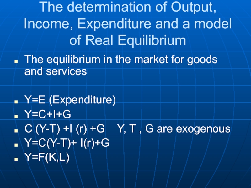
The equilibrium in the market for goods and services
Y=E (Expenditure)
Y=C+I+G
C (Y-T) +I (r) +G Y, T , G are exogenous
Y=C(Y-T)+ I(r)+G
Y=F(K,L)
Слайд 48The determination of Output, Income, Expenditure and a model of Real
The equilibrium in the financial market: the role of the interest rate
A) Savings
S=Y-C-G
S=(Y-T-G) +(T-G)
(Y-T-C)- private savings
(T-G) –public savings
Слайд 49The determination of Output, Income, Expenditure and a model of Real
The equilibrium in the financial market: the role of the interest rate
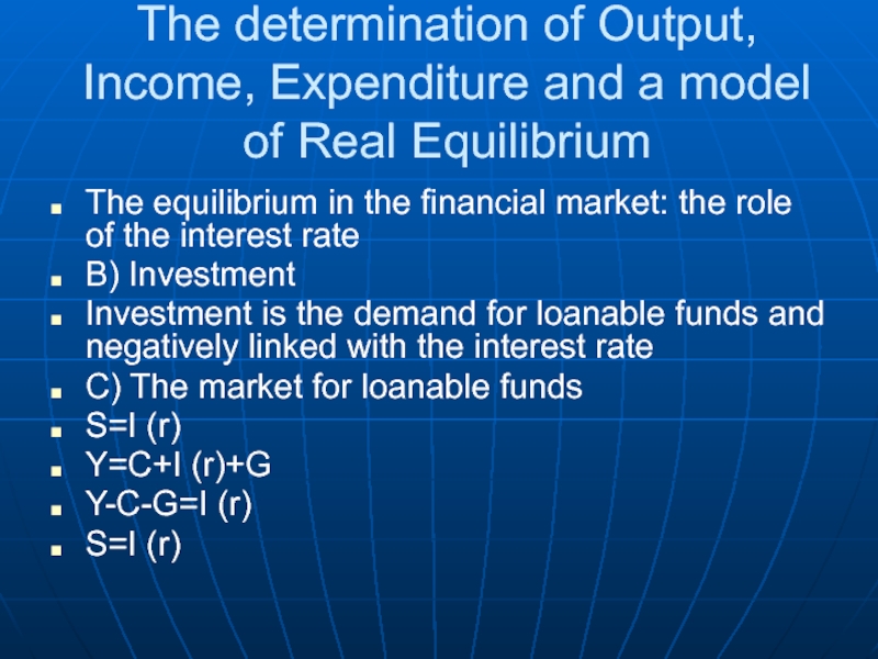
B) Investment
Investment is the demand for loanable funds and negatively linked with the interest rate
C) The market for loanable funds
S=I (r)
Y=C+I (r)+G
Y-C-G=I (r)
S=I (r)
Слайд 50The determination of Output, Income, Expenditure and a model of Real
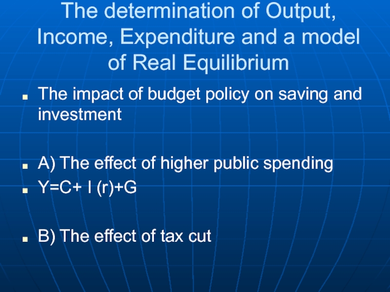
The impact of budget policy on saving and investment
A) The effect of higher public spending
Y=C+ I (r)+G
B) The effect of tax cut
Слайд 51Money, prices and interest rates
What is the impact of change in
What connection is there between the interest rate, demand for money and price trends
What problems between too large fluctuations in the price level.
Слайд 52Money, prices and interest rates
Money is one of the asset which
3 Functions of money
Money is a store of value.
Money is a unit of account, a measurement standard.
Money is an instrument of payment
Слайд 53Money, prices and interest rates
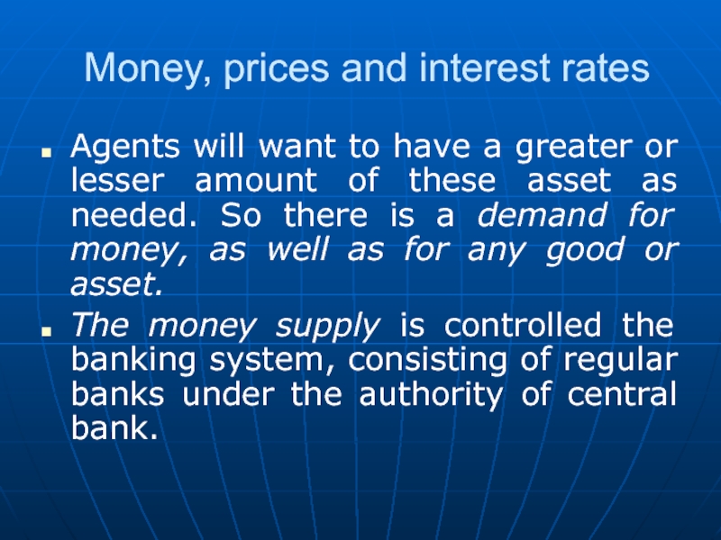
Agents will want to have a greater
The money supply is controlled the banking system, consisting of regular banks under the authority of central bank.
Слайд 54Money, prices and interest rates
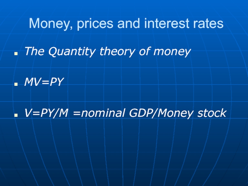
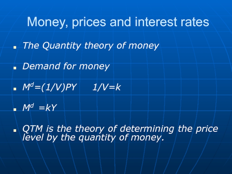
The Quantity theory of money
MV=PY
V=PY/M
Слайд 55Money, prices and interest rates
The Quantity theory of money
Demand for
Md=(1/V)PY 1/V=k
Md =kY
QTM is the theory of determining the price level by the quantity of money.
Слайд 56Money, prices and interest Rates
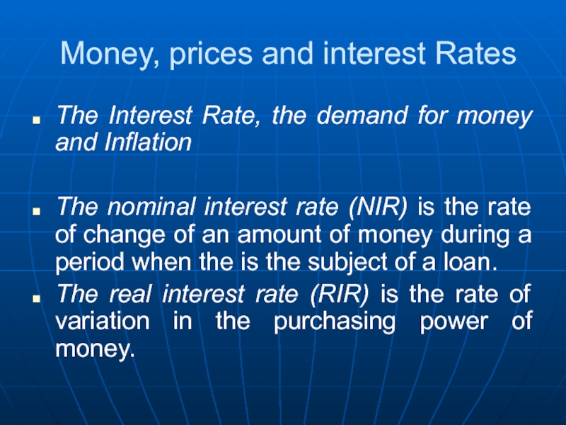
The Interest Rate, the demand for money
The nominal interest rate (NIR) is the rate of change of an amount of money during a period when the is the subject of a loan.
The real interest rate (RIR) is the rate of variation in the purchasing power of money.
Слайд 57Money, prices and interest Rates
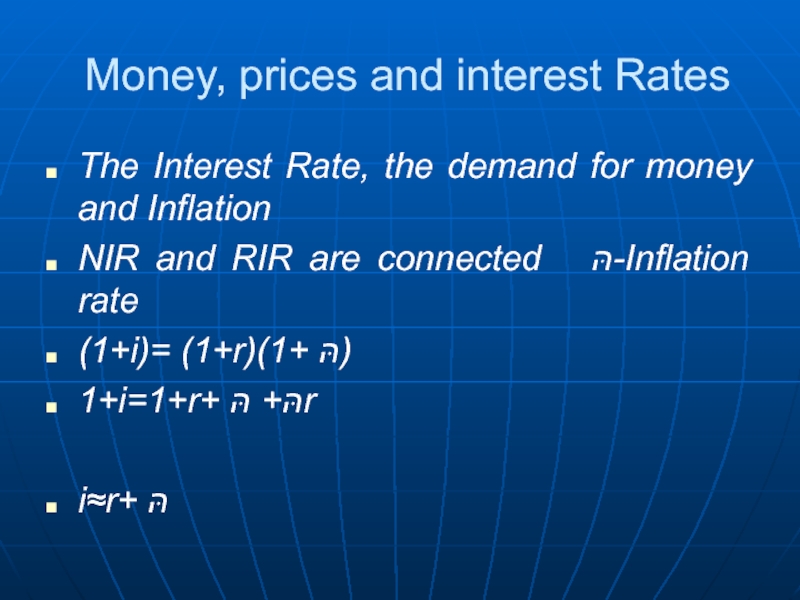
The Interest Rate, the demand for money
NIR and RIR are connected הּ-Inflation rate
(1+i)= (1+r)(1+ הּ)
1+i=1+r+ הּ+ הּr
i≈r+ הּ
Слайд 58Money, prices and interest Rates
The Interest Rate, the demand for money
NIR depends on:
-the real interest rate, itself determined between savings and investment
- expected inflation
i=r+הּe
Слайд 59Money, prices and interest Rates
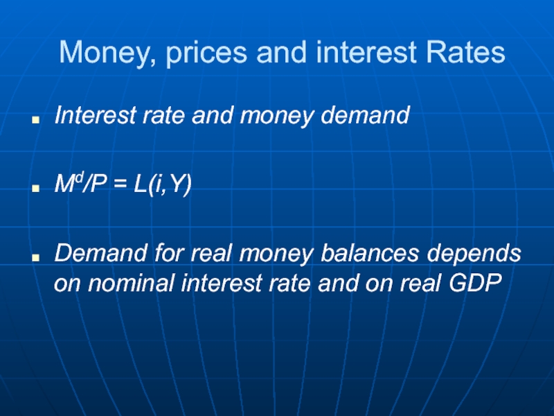
Interest rate and money demand
Md/P =
Demand for real money balances depends on nominal interest rate and on real GDP
Слайд 60Money, prices and interest Rates
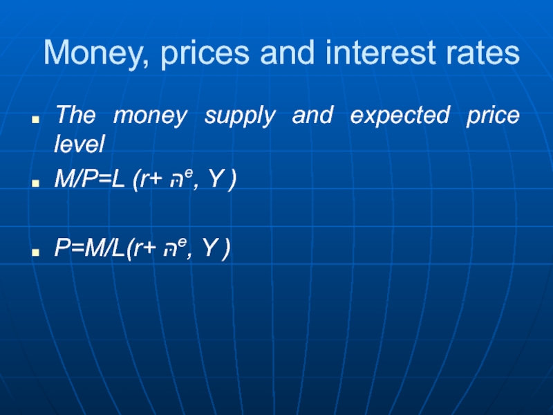
The money supply and expected price level
M/P
M/P=L (i, Y)
Слайд 61Money, prices and interest rates
The money supply and expected price level
M/P=L
P=M/L(r+ הּe, Y )
Слайд 62Money, prices and interest rates
The Problems with Too Large Fluctuation in
Inflation is a general rise in prices of goods and services.
Its effects on money functions
Inflation creates many distortions
Слайд 63Money, prices and interest rates
The Problems with Too Large Fluctuation in
Deflation is the symmetrical situation of inflation.
Слайд 64Labour market, employment, unemployment
Labour demand comes from com-panies that want to
Labour supply comes from indi-viduals who wish to earn an income.
Слайд 65Labour market, employment, unemployment
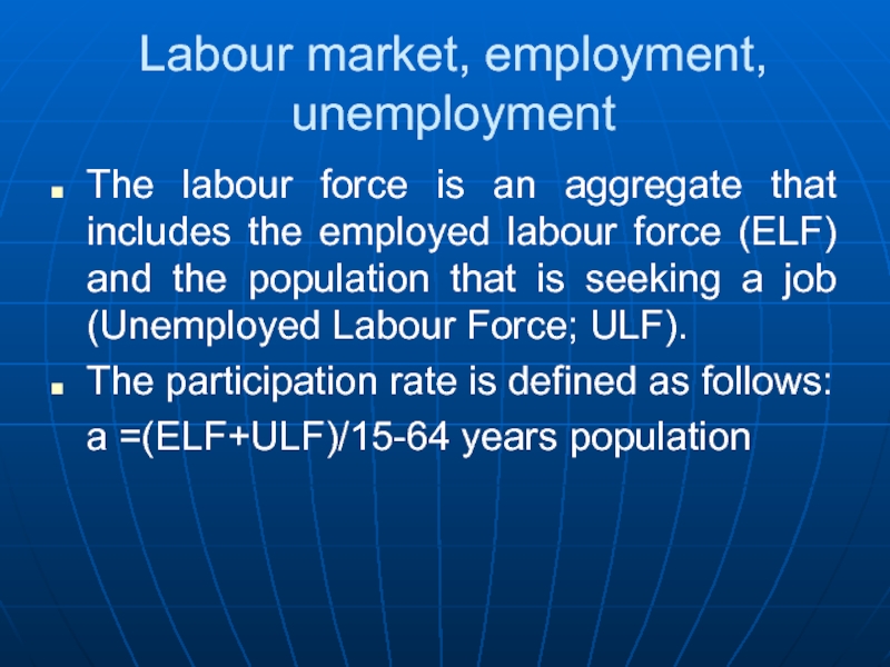
The labour force is an aggregate that includes
The participation rate is defined as follows:
a =(ELF+ULF)/15-64 years population
Слайд 66Labour market, employment, unemployment
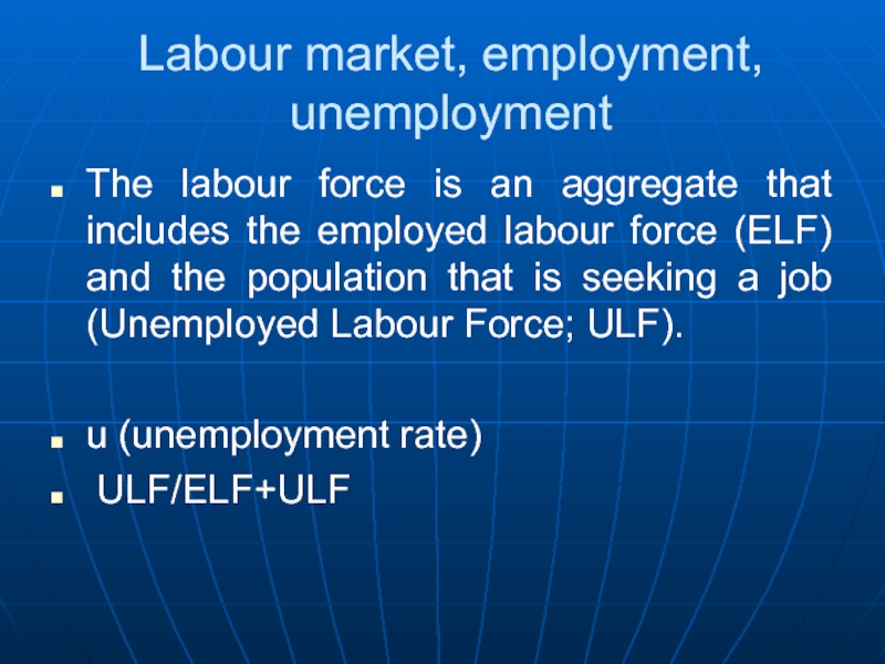
The labour force is an aggregate that includes
u (unemployment rate)
ULF/ELF+ULF
Слайд 67Labour market, employment, unemployment
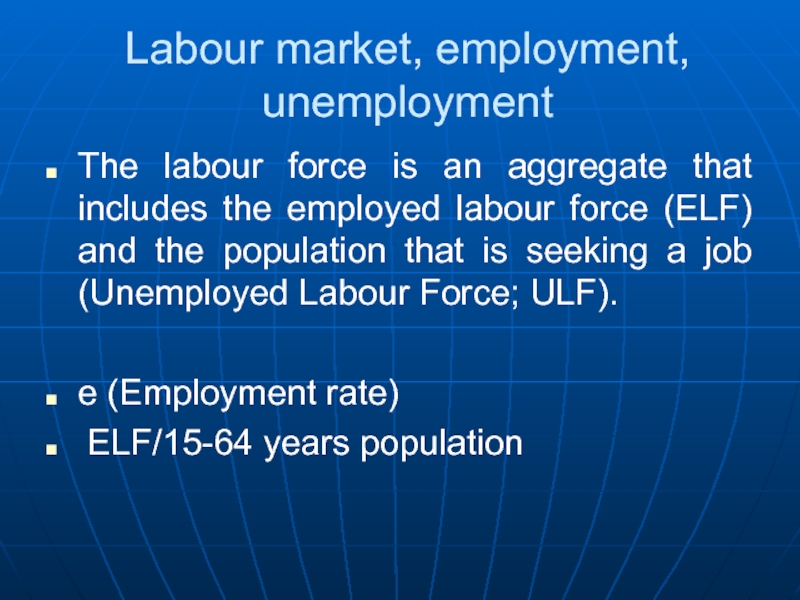
The labour force is an aggregate that includes
e (Employment rate)
ELF/15-64 years population
Слайд 68Labour market, employment, unemployment
N=E+U+I N=15-64 years old
a= (E+U)/N
e=E/N
u=U/(E+U)
a=e/(1-u)
Слайд 69Labour market, employment, unemployment
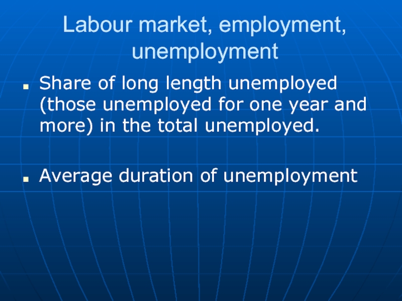
Share of long length unemployed (those unemployed for
Average duration of unemployment
Слайд 70Labour market, employment, unemployment
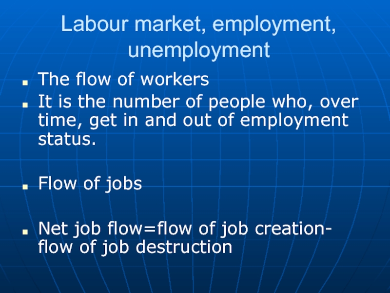
The flow of workers
It is the number of
Flow of jobs
Net job flow=flow of job creation- flow of job destruction
Слайд 71The Long-Run Rate of Unemployment
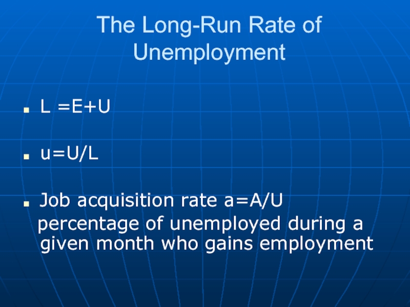
L =E+U
u=U/L
Job acquisition rate a=A/U
percentage of unemployed during a given month who gains employment
Слайд 72The Long-Run Rate of Unemployment
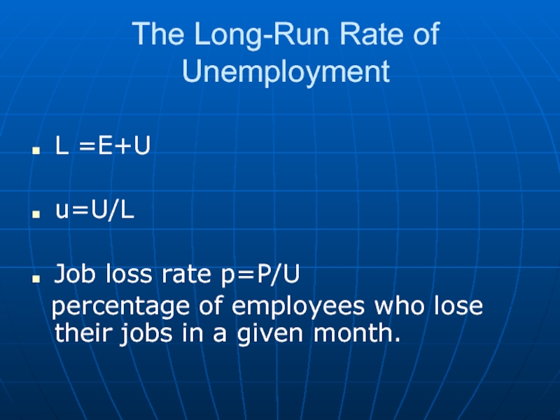
L =E+U
u=U/L
Job loss rate p=P/U
percentage of employees who lose their jobs in a given month.
Слайд 73The Long-Run Rate of Unemployment
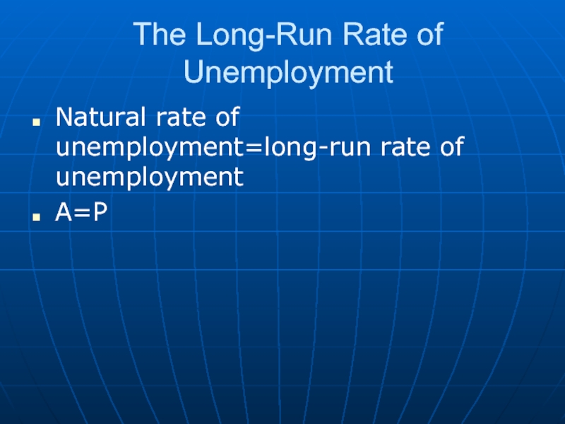
Natural rate of unemployment=long-run rate of unemployment
A=P
Слайд 74
Economic fluctuations
The economy is experiencing fluctuations that result in variations in
Слайд 75
Economic fluctuations
Acceleration phases (economic boom)
Contraction phase (economic recession)
Слайд 76
Economic fluctuations
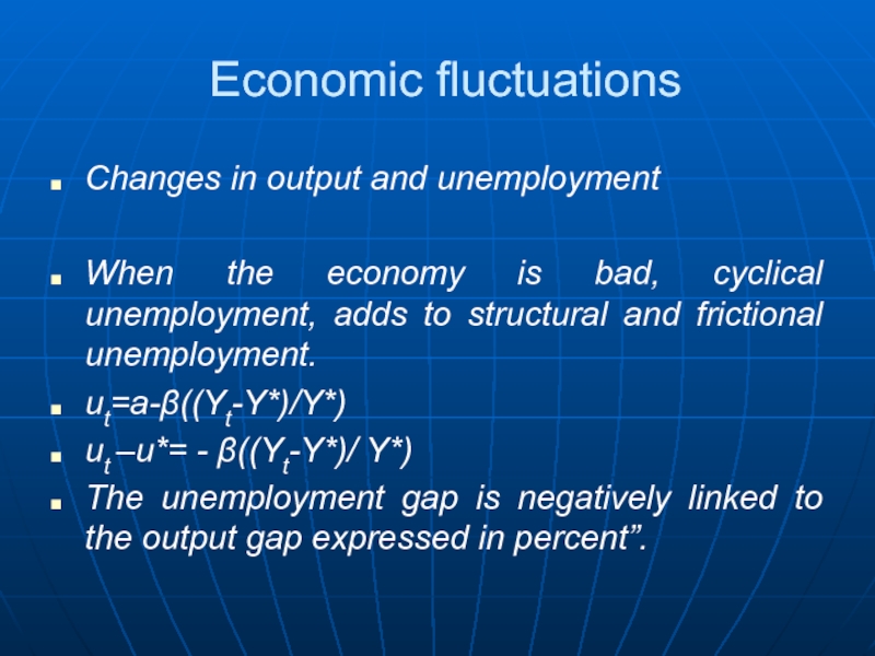
Changes in output and unemployment
When the economy is bad,
The relationship between output level and unemployment is known as “Okun,s law”
Слайд 77
Economic fluctuations
Changes in output and unemployment
When the economy is bad,
Okun consider that: the unemployment rate is negatively linked to the level of output.
Слайд 78
Economic fluctuations
Changes in output and unemployment
When the economy is bad,
ut=a-β((Yt-Y*)/Y*)
ut –u*= - β((Yt-Y*)/ Y*)
The unemployment gap is negatively linked to the output gap expressed in percent”.
Слайд 79
Economic fluctuations
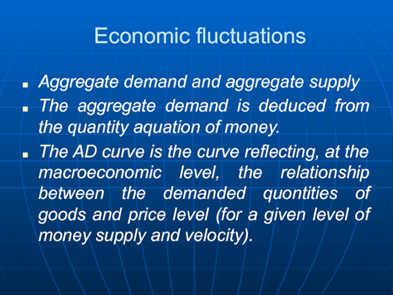
Aggregate demand and aggregate supply
The aggregate demand is deduced
The AD curve is the curve reflecting, at the macroeconomic level, the relationship between the demanded quontities of goods and price level (for a given level of money supply and velocity).
Слайд 80
Economic fluctuations
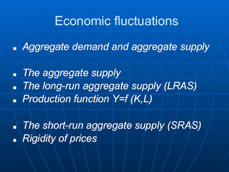
Aggregate demand and aggregate supply
The aggregate supply
The long-run aggregate
Production function Y=f (K,L)
The short-run aggregate supply (SRAS)
Rigidity of prices
Слайд 81
Economic fluctuations
Aggregate demand and aggregate supply
AS-AD model
Long-run effect of change
In the long run only the price level is effected.
Слайд 82
Economic fluctuations
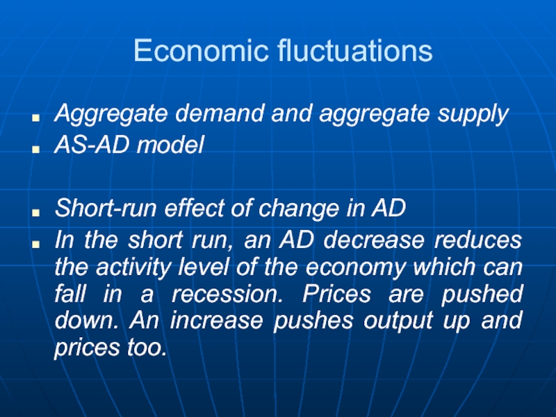
Aggregate demand and aggregate supply
AS-AD model
Short-run effect of change
In the short run, an AD decrease reduces the activity level of the economy which can fall in a recession. Prices are pushed down. An increase pushes output up and prices too.
Слайд 83
Economic fluctuations
Aggregate demand and aggregate supply
AS-AD model
The Effect of Monetary
The Central bank can reduce the money supply
The M decrease reduces AD, which affects the level of output Y and the economy enters a recession.
Over time, given the weak demand, prices will decrease. The prices decrease brings the economy towards its long-run equilibrium.
Слайд 84
Economic fluctuations
Aggregate demand and aggregate supply
AS-AD model
The Effect of Monetary
1) a decrease in output in the short run, then a return to the long-run value
2) price stability in the short run and lower prices over time
Слайд 85
Economic fluctuations
Aggregate demand and aggregate supply
AS-AD model
The Effect of Monetary
1) a decrease in output in the short run, then a return to the long-run value
2) price stability in the short run and lower prices over time
Слайд 86
Economic fluctuations
Aggregate demand and aggregate supply
AS-AD model
The Effect of Monetary
1) a decrease in output in the short run, then a return to the long-run value
2) price stability in the short run and lower prices over time
Слайд 87
Economic fluctuations
External shock –an event that affects suddenly the economy and
Demand shocks affect the main components of demand: con-sumption, investment, exports.
Supply shocks cause changes in production costs for firms.
Слайд 88The Keynesian Model of Short-Run Equilibrium
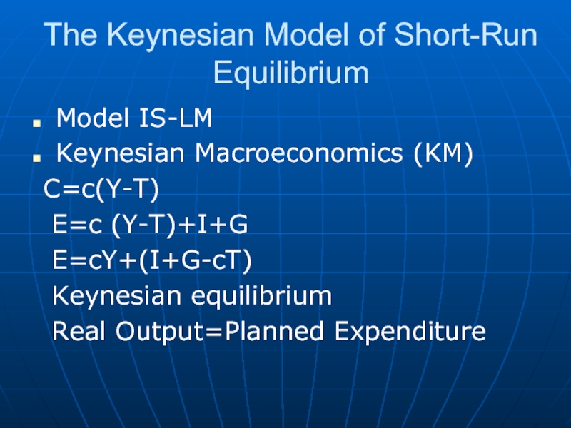
Model IS-LM
Keynesian Macroeconomics (KM)
-
- the short run equilibrium does not necessarily correspond to full employment and the level of employment is determined by the level of aggregate demand
- the quantity of money has an impact on the level of real output
Слайд 89The Keynesian Model of Short-Run Equilibrium
Model IS-LM
Keynesian Macroeconomics (KM)
E=c (Y-T)+I+G
E=cY+(I+G-cT)
Keynesian equilibrium
Real Output=Planned Expenditure
Слайд 90The Keynesian Model of Short-Run Equilibrium
Model IS-LM
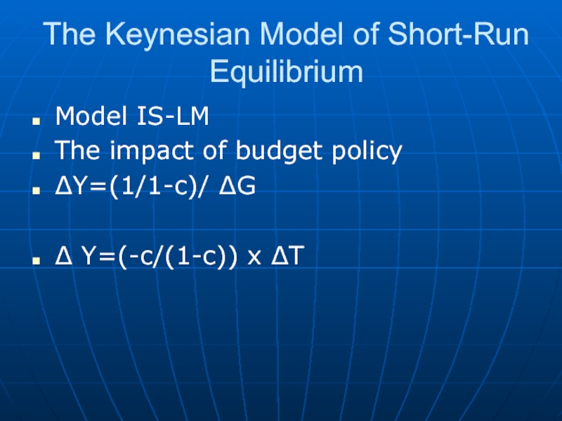
The impact of budget
∆Y=(1/1-c)/ ∆G
∆ Y=(-c/(1-c)) x ∆T
Слайд 91The Keynesian Model of Short-Run Equilibrium
Model IS-LM
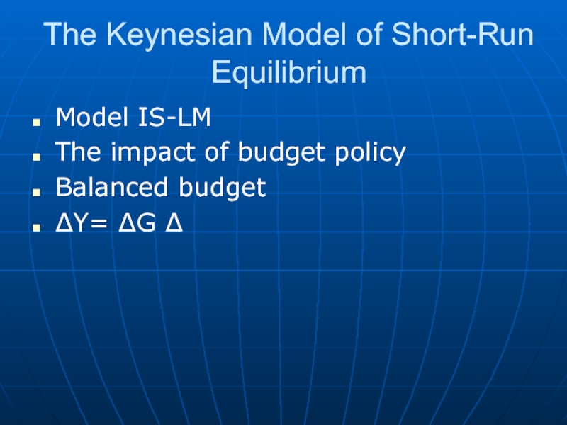
The impact of budget
Balanced budget
∆Y= ∆G ∆
Слайд 92The Keynesian Model of Short-Run Equilibrium
Model IS-LM
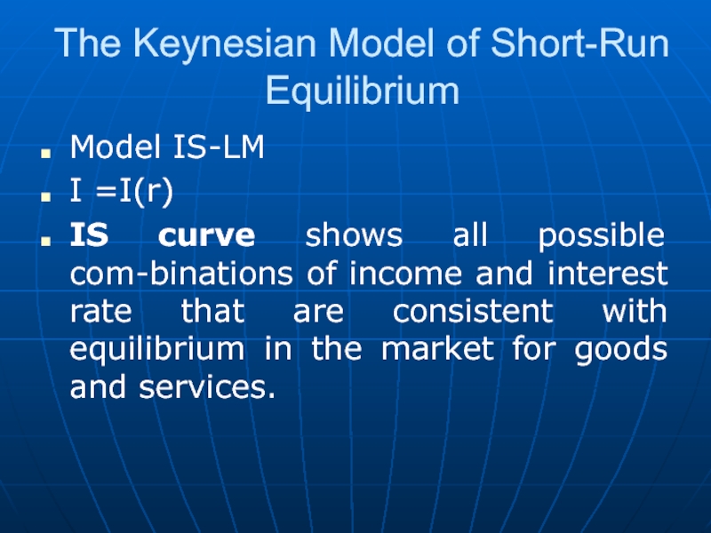
I =I(r)
IS curve
Слайд 93The Keynesian Model of Short-Run Equilibrium
Model IS-LM
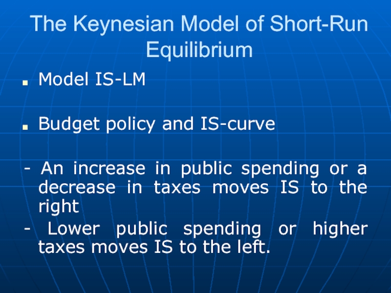
Budget policy and IS-curve
- An increase in public spending or a decrease in taxes moves IS to the right
- Lower public spending or higher taxes moves IS to the left.
Слайд 94The Keynesian Model of Short-Run Equilibrium
Model IS-LM
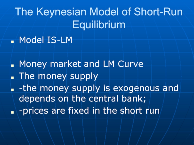
Money market and LM
The money supply
-the money supply is exogenous and depends on the central bank;
-prices are fixed in the short run
Слайд 95The Keynesian Model of Short-Run Equilibrium
Model IS-LM
Money market and LM
The demand for money
Md/P=L(i,Y)
- transaction motive
- a care motive
- speculative motive
Слайд 96The Keynesian Model of Short-Run Equilibrium
Model IS-LM
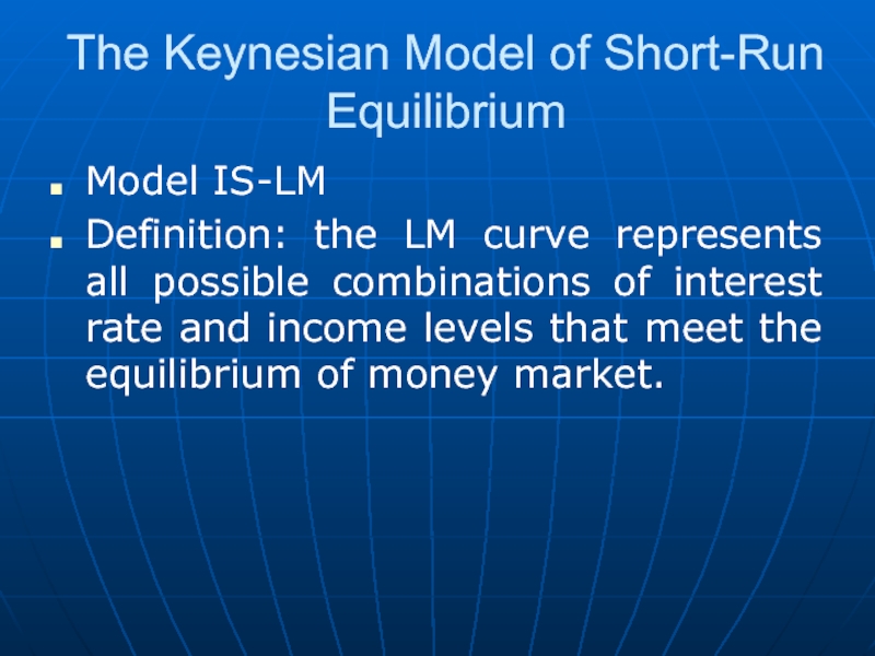
Definition: the LM curve
Слайд 97The Keynesian Model of Short-Run Equilibrium
Model IS-LM
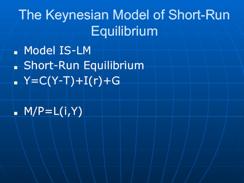
Short-Run Equilibrium
Y=C(Y-T)+I(r)+G
M/P=L(i,Y)
Слайд 98The Keynesian Model of Short-Run Equilibrium
Model IS-LM
Economic Policy through the
The stabilization of the economy through budget policy
-The case of a rise in public spending
-The case of tax-cut
Слайд 99The Keynesian Model of Short-Run Equilibrium
Model IS-LM
Economic Policy through the
The stabilization of activity by monetary policy
The interaction of budget and monetary policies
Слайд 100The Keynesian Model of Short-Run Equilibrium
Model IS-LM
IS-LM and aggregate demand
IS-LM
Слайд 101Aggregate Supply
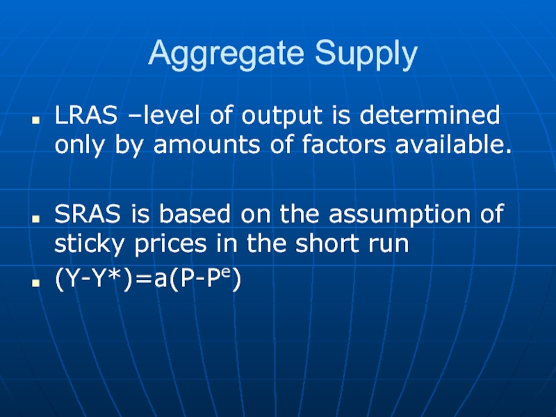
LRAS –level of output is determined only by amounts of
SRAS is based on the assumption of sticky prices in the short run
(Y-Y*)=a(P-Pe)
Слайд 103Aggregate Supply
The effect of a change in prices expectations
Y=Y*+a(P-Pe)
u=u* הּ= הּ-1
When
Phillips-curve.

