- Главная
- Разное
- Дизайн
- Бизнес и предпринимательство
- Аналитика
- Образование
- Развлечения
- Красота и здоровье
- Финансы
- Государство
- Путешествия
- Спорт
- Недвижимость
- Армия
- Графика
- Культурология
- Еда и кулинария
- Лингвистика
- Английский язык
- Астрономия
- Алгебра
- Биология
- География
- Детские презентации
- Информатика
- История
- Литература
- Маркетинг
- Математика
- Медицина
- Менеджмент
- Музыка
- МХК
- Немецкий язык
- ОБЖ
- Обществознание
- Окружающий мир
- Педагогика
- Русский язык
- Технология
- Физика
- Философия
- Химия
- Шаблоны, картинки для презентаций
- Экология
- Экономика
- Юриспруденция
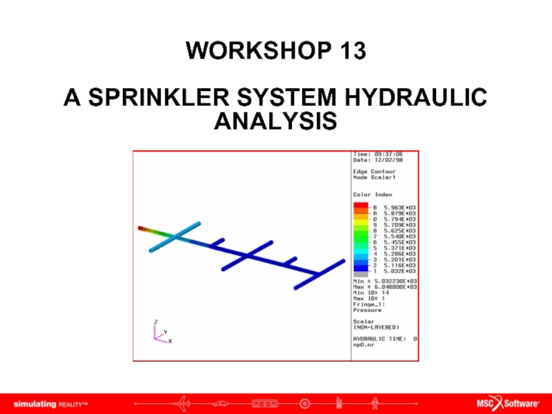
WORKSHOP 13 A SPRINKLER SYSTEM HYDRAULIC ANALYSIS презентация
Содержание
- 1. WORKSHOP 13 A SPRINKLER SYSTEM HYDRAULIC ANALYSIS
- 3. Model Description In this exercise you will
- 4. Exercise Overview Create a new database named
- 5. Step 1: Create a New Database Create
- 6. Step 2: Create Network Schematic Geometry Create
- 7. Step 2: Create Network Schematic Geometry (Cont.)
- 8. Step 2: Create Network Schematic Geometry (Cont.)
- 9. Step 2: Create Network Schematic Geometry (Cont.)
- 10. Step 2: Create Network Schematic Geometry (Cont.)
- 11. Step 3: Create Nodes and Elements Create
- 12. b c d e Continue creating FEM
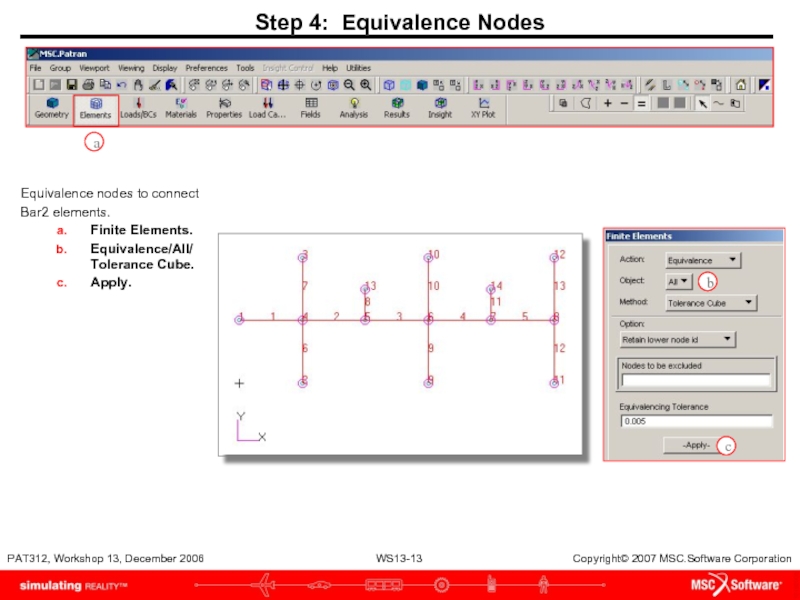
- 13. Step 4: Equivalence Nodes Equivalence nodes to
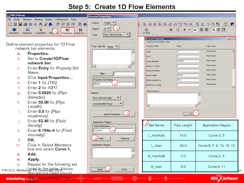
- 14. Step 5: Create 1D Flow Elements Define
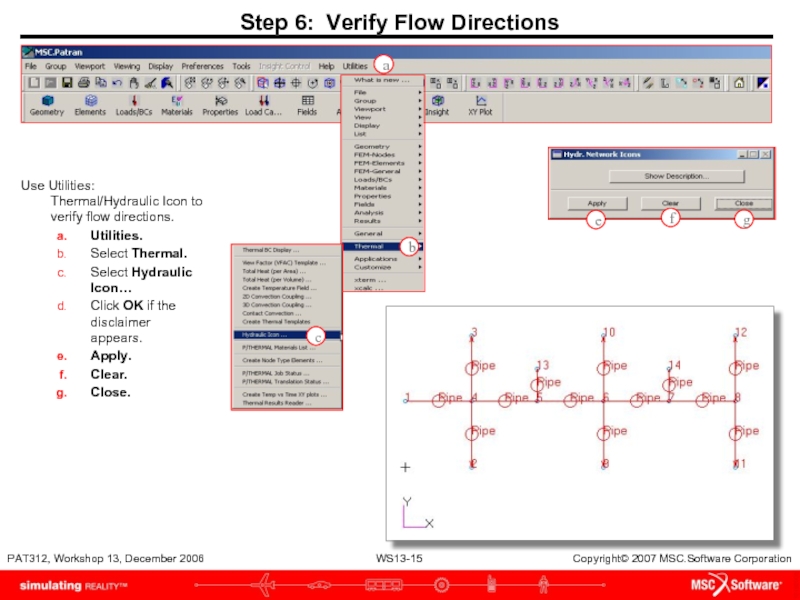
- 15. Step 6: Verify Flow Directions Use Utilities:
- 16. Step 7: Create Micro-Functions/Fields Create first NonSpatial
- 17. Create second NonSpatial fields which defines the
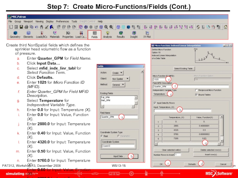
- 18. Create third NonSpatial fields which defines the
- 19. Step 8: Apply Boundary Conditions Define inlet
- 20. Step 8: Apply Boundary Conditions (Cont.) Create
- 21. Step 8: Apply Boundary Conditions (Cont.) Repeat
- 22. Step 8: Apply Boundary Conditions (Cont.) Repeat
- 23. Step 8: Apply Boundary Conditions (Cont.) Change
- 24. Step 9: Create template.dat.apnd File Use Analysis:
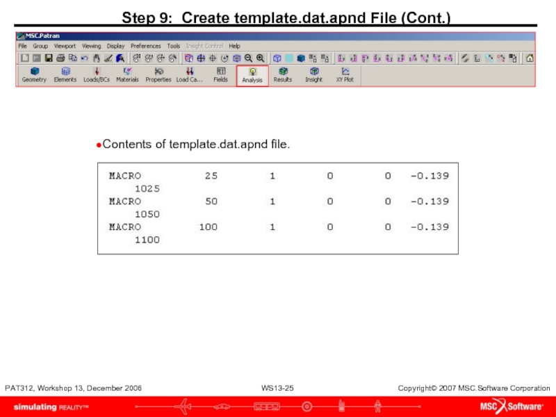
- 25. Step 9: Create template.dat.apnd File (Cont.) Contents of template.dat.apnd file.
- 26. Step 10: Prepare and Run Analysis Prepare
- 27. Step 11: Read and Plot Results Read
- 28. Step 11: Read and Plot Results (Cont.)
- 29. Step 11: Read and Plot Results (Cont.)
- 30. Step 11: Read and Plot Results (Cont.)
- 31. Step 12: Quit MSC.Patran Quit MSC.Patran.
Слайд 3Model Description
In this exercise you will create schematic geometry which models
The home for which this sprinkler is designed can comfortably deliver 12 gallons per minute (GPM) of water at 42 psi through the existing main. Since both the volumetric flow through and the coverage from each sprinkler head are a function of pressure at the head, this analysis will determine whether the pressure at each head is above 30 psi and whether the entry volumetric flow demand is less that 12 GPM.
All data provided yield an analysis in English Engineering units, lbf, lbm, s, feet. However here are some useful conversion factors for evaluating the results: 1 cu. Ft. = 7.481 gal. And 1 sq. ft. = 144 sq. in.
Слайд 4Exercise Overview
Create a new database named exercise_13.db. Set Tolerance to Default,
Create flow network schematic geometry using the Geometry form Create and Transform Actions.
Create FEM entities. Create nodes matching geometric points and mesh curve with BAR2 elements.
Equivalence nodes.
Define element properties for 1D Flow network bar elements using IOPT=2 for automatic friction factor calculation.
Use Utilities/Thermal/Hydraulic Icon to check flow direction.
Create three NonSpatial/General fields which define the sprinkler head volumetric flow as a function of pressure.
Define inlet pressure and sprinkler head mass flow conditions.
Use Analysis/Build Template to create the template.dat.apnd file.
Select Analysis to prepare and to submit the model for analysis and to Read Results.
Run the analysis and read the results into the database.
Quit MSC/PATRAN.
Objectives
Model a schematic of a home sprinkler system.
Use microfunctions to apply pressure varying mass flow functions at the sprinkler heads.
Run a hydraulic analysis to evaluate the pressure drop and total mass flow through the system.
Слайд 5Step 1: Create a New Database
Create a new database called exercise_13.db.
File
Enter exercise_13 as the file name.
Click OK.
Choose Default Tolerance.
Select MSC.Thermal as the Analysis Code.
Select Thermal as the Analysis Type.
OK.
a
b
c
d
e
f
g
Слайд 6Step 2: Create Network Schematic Geometry
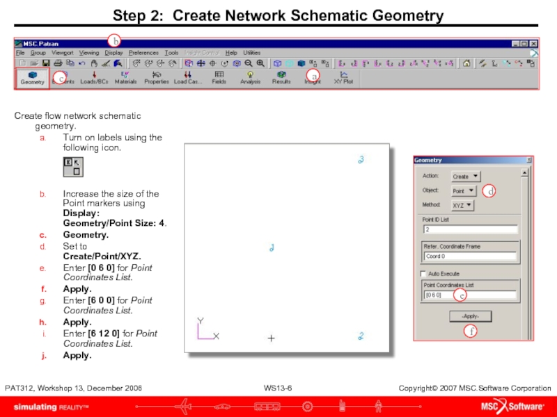
Create flow network schematic geometry.
Turn on
Increase the size of the Point markers using Display: Geometry/Point Size: 4.
Geometry.
Set to Create/Point/XYZ.
Enter [0 6 0] for Point Coordinates List.
Apply.
Enter [6 0 0] for Point Coordinates List.
Apply.
Enter [6 12 0] for Point Coordinates List.
Apply.
a
d
e
f
b
c
Слайд 7Step 2: Create Network Schematic Geometry (Cont.)
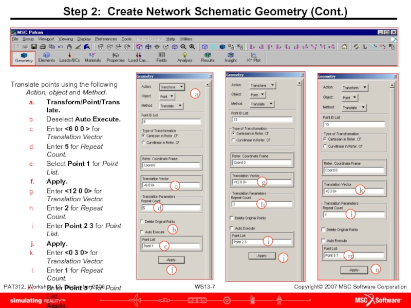
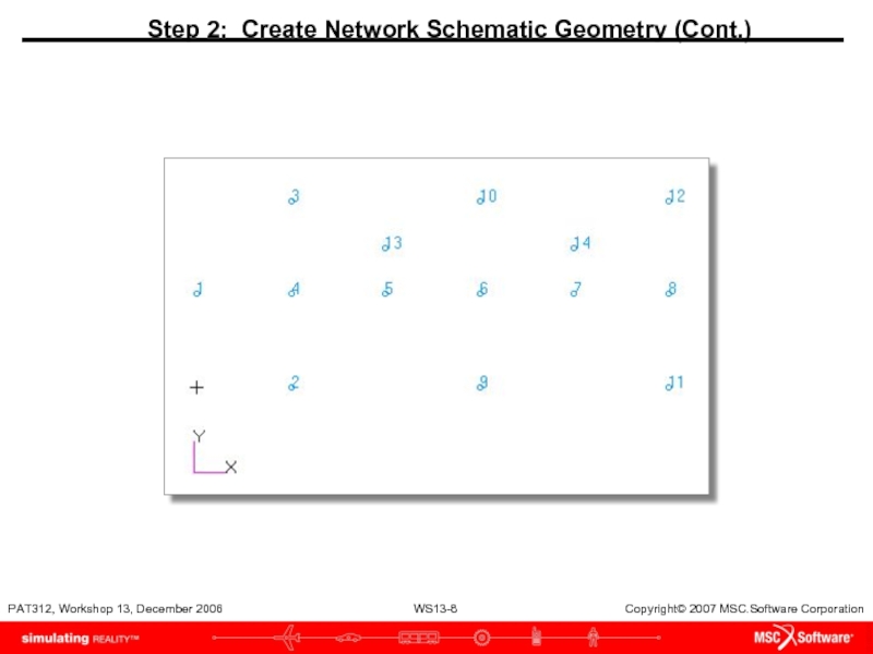
Translate points using the following
Transform/Point/Translate.
Deselect Auto Execute.
Enter <6 0 0 > for Translation Vector.
Enter 5 for Repeat Count.
Select Point 1 for Point List.
Apply.
Enter <12 0 0> for Translation Vector.
Enter 2 for Repeat Count.
Enter Point 2 3 for Point List.
Apply.
Enter <0 3 0> for Translation Vector.
Enter 1 for Repeat Count.
Enter Point 5 7 for Point List.
Apply.
Слайд 9Step 2: Create Network Schematic Geometry (Cont.)
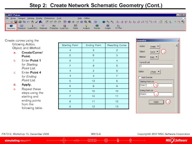
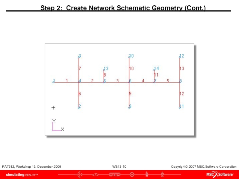
Create curves using the following
Create/Curve/Point.
Enter Point 1 for Starting Point List.
Enter Point 4 for Ending Point List.
Apply.
Repeat these steps using the starting and ending points from the following table.
a
b
c
d
Слайд 11Step 3: Create Nodes and Elements
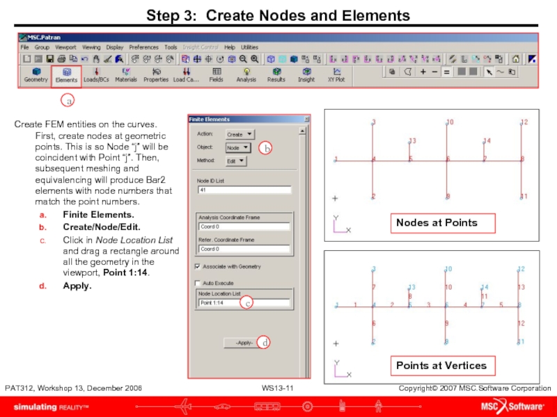
Create FEM entities on the curves.
Finite Elements.
Create/Node/Edit.
Click in Node Location List and drag a rectangle around all the geometry in the viewport, Point 1:14.
Apply.
a
b
c
d
Nodes at Points
Points at Vertices
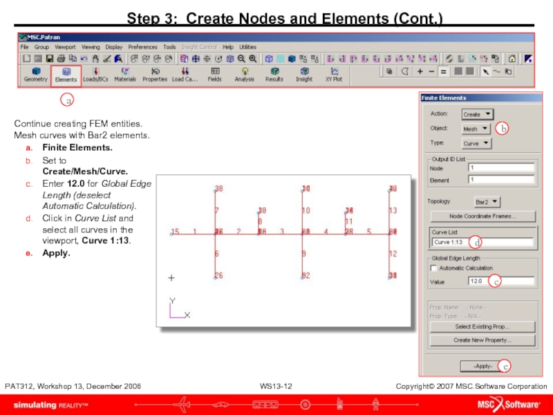
Слайд 12b
c
d
e
Continue creating FEM entities. Mesh curves with Bar2 elements.
Finite Elements.
Set to
Enter 12.0 for Global Edge Length (deselect Automatic Calculation).
Click in Curve List and select all curves in the viewport, Curve 1:13.
Apply.
Step 3: Create Nodes and Elements (Cont.)
a
Слайд 13Step 4: Equivalence Nodes
Equivalence nodes to connect
Bar2 elements.
Finite Elements.
Equivalence/All/ Tolerance
Apply.
a
b
c
Слайд 14Step 5: Create 1D Flow Elements
Define element properties for 1D Flow
Properties.
Set to Create/1D/Flow network bar.
Enter Entry for Property Set Name.
Click Input Properties…
Enter 1 for [TID].
Enter 2 for IOPT.
Enter 0.0625 for [Pipe diameter].
Enter 50.00 for [Pipe Length].
Enter 0.0 for [Pipe roughness].
Enter 62.46 for [Fluid density].
Enter 6.764e-4 for [Fluid viscosity].
OK.
Click in Select Members box and select Curve 1.
Add.
Apply.
Repeat for the following set listed in the table. Values that are not listed should stay untouched (left the same).
a
b
c
d
l
m
o
p
n
Слайд 15Step 6: Verify Flow Directions
Use Utilities: Thermal/Hydraulic Icon to verify flow
Utilities.
Select Thermal.
Select Hydraulic Icon…
Click OK if the disclaimer appears.
Apply.
Clear.
Close.
a
b
c
e
f
g
Слайд 16Step 7: Create Micro-Functions/Fields
Create first NonSpatial fields which defines the sprinkler
Fields.
Create/Non Spatial/General.
Enter Full_GPM for Field Name.
Click Input Data…
Select mfid_indx_linr_tabl for Select Function Term.
Enter 1100 for Micro Function ID (MFID).
Enter Full_GPM for Field MFID Description.
Select Temperature for Independent Variable Type.
Enter 0.0 for Input: Temperature (X).
Enter 0.0 for Input: Value, Function (X).
Enter 2880.0 for Input: Temperature (X).
Enter 1.67 for Input: Value, Function (X).
Enter 4320.0 for Input: Temperature (X).
Enter 2.19 for Input: Value, Function (X).
Enter 5760.0 for Input: Temperature (X).
Enter 2.35 for Input: Value, Function (X).
Enter 7200.0 for Input: Temperature (X).
Enter 2.7 for Input: Value, Function (X).
Click OK, OK and Apply.
a
b
c
d
f
h
s
g
Слайд 17Create second NonSpatial fields which defines the sprinkler head volumetric flow
Enter Half_GPM for Field Name.
Click Input Data…
Select mfid_indx_linr_tabl for Select Function Term.
Select Defaults to clear the form.
Enter 1050 for Micro Function ID (MFID).
Enter Half_GPM for Field MFID Description.
Select Temperature for Independent Variable Type.
Enter 0.0 for Input: Temperature (X).
Enter 0.0 for Input: Value, Function (X).
Enter 2880.0 for Input: Temperature (X).
Enter 0.95 for Input: Value, Function (X).
Enter 4320.0 for Input: Temperature (X).
Enter 1.09 for Input: Value, Function (X).
Enter 5760.0 for Input: Temperature (X).
Enter 1.3 for Input: Value, Function (X).
Enter 7200.0 for Input: Temperature (X).
Enter 1.55 Input: Value, Function (X).
Click OK, OK, then Apply.
a
b
e
f
q
d
g
h
r
Step 7: Create Micro-Functions/Fields (Cont.)
Слайд 18Create third NonSpatial fields which defines the sprinkler head volumetric flow
Enter Quarter_GPM for Field Name.
Click Input Data…
Select mfid_indx_linr_tabl for Select Function Term.
Click Defaults.
Enter 1025 for Micro Function ID (MFID).
Enter Quarter_GPM for Field MFID Description.
Select Temperature for Independent Variable Type.
Enter 0.0 for Input: Temperature (X).
Enter 0.0 for Input: Value, Function (X).
Enter 2880.0 for Input: Temperature (X).
Enter 0.40 for Input: Value, Function (X).
Enter 4320.0 for Input: Temperature (X).
Enter 0.50 for Input: Value, Function (X).
Enter 5760.0 for Input: Temperature (X).
Enter 0.60 for Input: Value, Function (X).
Enter 7200.0 for Input: Temperature (X).
Enter 0.63 for Input: Value, Function (X).
Click OK, OK, then Apply.
e
b
a
f
q
d
g
h
r
Step 7: Create Micro-Functions/Fields (Cont.)
Слайд 19Step 8: Apply Boundary Conditions
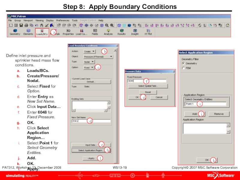
Define inlet pressure and sprinkler head mass
Loads/BCs.
Create/Pressure/Nodal.
Select Fixed for Option.
Enter Entry as New Set Name.
Click Input Data…
Enter 6048 for Fixed Pressure.
OK.
Click Select Application Region…
Select Point 1 for Select Geometry Entities.
Add.
OK.
Apply.
a
b
c
d
e
f
g
h
i
k
l
j
Слайд 20Step 8: Apply Boundary Conditions (Cont.)
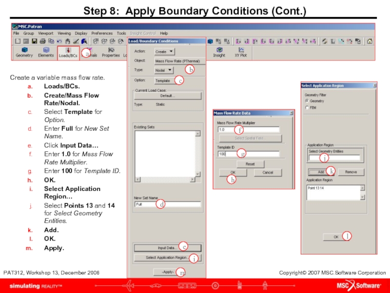
Create a variable mass flow rate.
Loads/BCs.
Create/Mass
Select Template for Option.
Enter Full for New Set Name.
Click Input Data…
Enter 1.0 for Mass Flow Rate Multiplier.
Enter 100 for Template ID.
OK.
Select Application Region…
Select Points 13 and 14 for Select Geometry Entities.
Add.
OK.
Apply.
a
b
c
d
e
f
g
h
i
j
l
m
k
Слайд 21Step 8: Apply Boundary Conditions (Cont.)
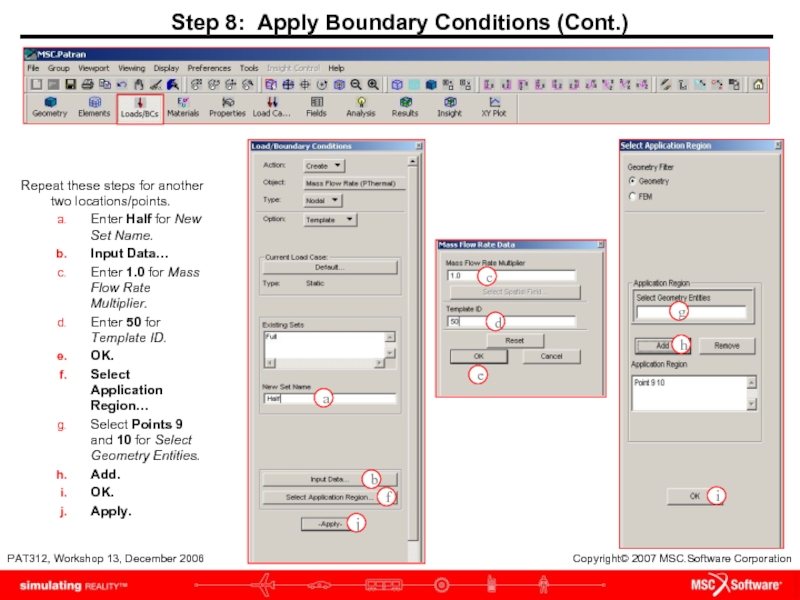
Repeat these steps for another two
Enter Half for New Set Name.
Input Data…
Enter 1.0 for Mass Flow Rate Multiplier.
Enter 50 for Template ID.
OK.
Select Application Region…
Select Points 9 and 10 for Select Geometry Entities.
Add.
OK.
Apply.
a
b
c
d
e
f
g
i
j
h
Слайд 22Step 8: Apply Boundary Conditions (Cont.)
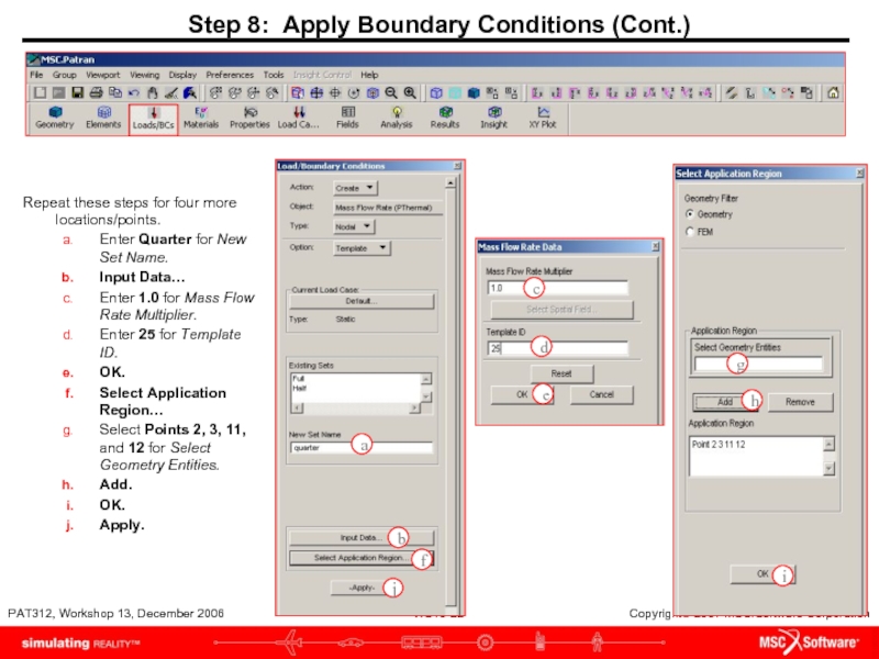
Repeat these steps for four more
Enter Quarter for New Set Name.
Input Data…
Enter 1.0 for Mass Flow Rate Multiplier.
Enter 25 for Template ID.
OK.
Select Application Region…
Select Points 2, 3, 11, and 12 for Select Geometry Entities.
Add.
OK.
Apply.
a
b
c
d
e
f
g
i
j
h
Слайд 23Step 8: Apply Boundary Conditions (Cont.)
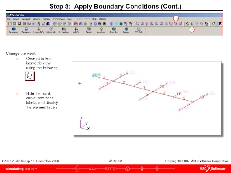
Change the view.
Change to the isometric
Hide the point, curve, and node labels, and display the element labels.
a
b
Слайд 24Step 9: Create template.dat.apnd File
Use Analysis: Build Template to create the
Analysis.
Build template.
Click Create Template File…
Create/MACRO/Data Entry.
Enter 25 for MACRO ID.
Enter 1025 for MFID’s.
Enter –0.139 for Scale Factor.
Apply.
Click Cancel in Template Entries form.
Repeat these steps with the information in the table.
After entering the last set of information do not cancel Template Entries form, but select Write File…
In the box for File name input template.dat.apnd.
OK.
Cancel.
Cancel.
a
Слайд 26Step 10: Prepare and Run Analysis
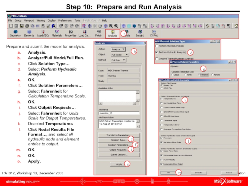
Prepare and submit the model for
Analysis.
Analyze/Full Model/Full Run.
Click Solution Type…
Select Perform Hydraulic Analysis.
OK.
Click Solution Parameters…
Select Fahrenheit for Calculation Temperature Scale.
OK.
Click Output Requests…
Select Fahrenheit for Units Scale for Output Temperatures.
Deselect Temperatures
Click Nodal Results File Format…, and select all hydraulic node and element entries to output.
OK.
OK.
Apply.
a
b
c
d
f
g
l
m
o
i
k
Слайд 27Step 11: Read and Plot Results
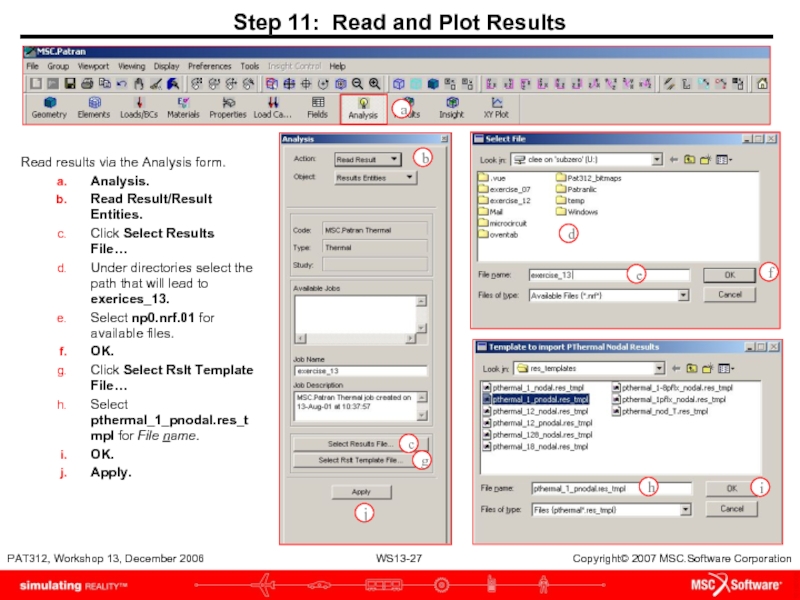
Read results via the Analysis form.
Analysis.
Read
Click Select Results File…
Under directories select the path that will lead to exerices_13.
Select np0.nrf.01 for available files.
OK.
Click Select Rslt Template File…
Select pthermal_1_pnodal.res_tmpl for File name.
OK.
Apply.
a
b
c
d
f
g
h
i
j
e
Слайд 28Step 11: Read and Plot Results (Cont.)
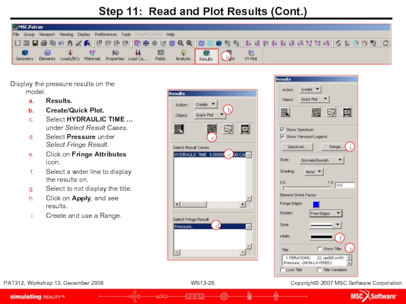
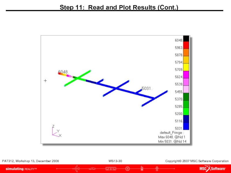
Display the pressure results on
Results.
Create/Quick Plot.
Select HYDRAULIC TIME … under Select Result Cases.
Select Pressure under Select Fringe Result.
Click on Fringe Attributes icon.
Select a wider line to display the results on.
Select to not display the title.
Click on Apply, and see results.
Create and use a Range.
b
i
e
c
g
f
d
a
Слайд 29Step 11: Read and Plot Results (Cont.)
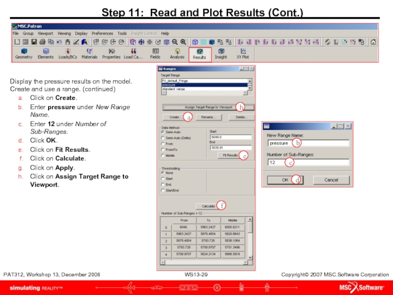
Display the pressure results on
Click on Create.
Enter pressure under New Range Name.
Enter 12 under Number of Sub-Ranges.
Click OK.
Click on Fit Results.
Click on Calculate.
Click on Apply.
Click on Assign Target Range to Viewport.
a
b
c
d
e
f
h
