- Главная
- Разное
- Дизайн
- Бизнес и предпринимательство
- Аналитика
- Образование
- Развлечения
- Красота и здоровье
- Финансы
- Государство
- Путешествия
- Спорт
- Недвижимость
- Армия
- Графика
- Культурология
- Еда и кулинария
- Лингвистика
- Английский язык
- Астрономия
- Алгебра
- Биология
- География
- Детские презентации
- Информатика
- История
- Литература
- Маркетинг
- Математика
- Медицина
- Менеджмент
- Музыка
- МХК
- Немецкий язык
- ОБЖ
- Обществознание
- Окружающий мир
- Педагогика
- Русский язык
- Технология
- Физика
- Философия
- Химия
- Шаблоны, картинки для презентаций
- Экология
- Экономика
- Юриспруденция
System reliability презентация
Содержание
- 1. System reliability
- 2. Definition It’s the probability of successful operation
- 3. Definition and Notation Reliability: R(t) = Probability
- 4. Definitions et notations Mean time before failures:
- 5. Definitions et notations Mean up time :
- 6. stochastic Processes Renewal process: We consider a
- 7. stochastic Processes We called variable renewal process
- 8. Fondamental relations We note by T
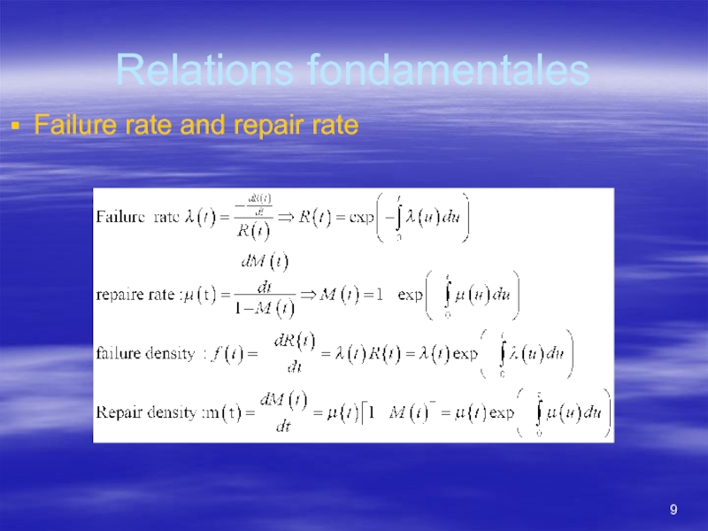
- 9. Relations fondamentales Failure rate and repair rate
- 10. Method of determination of the material failure
- 11. Method of determination of the material failure
- 12. Method of determination of the material failure
- 13. Method of determination of the material failure
- 14. Method of determination of the material failure law « New material » Case 2 N
- 15. Method of determination of the material failure law « New material » Case 2 N
- 16. Method of determination of the material failure
- 17. Acceptance test for obtained law Case
- 18. Acceptance test for obtained law Case
- 19. Principal law used in industry and research in reliability frame
- 20. Usuel discret law
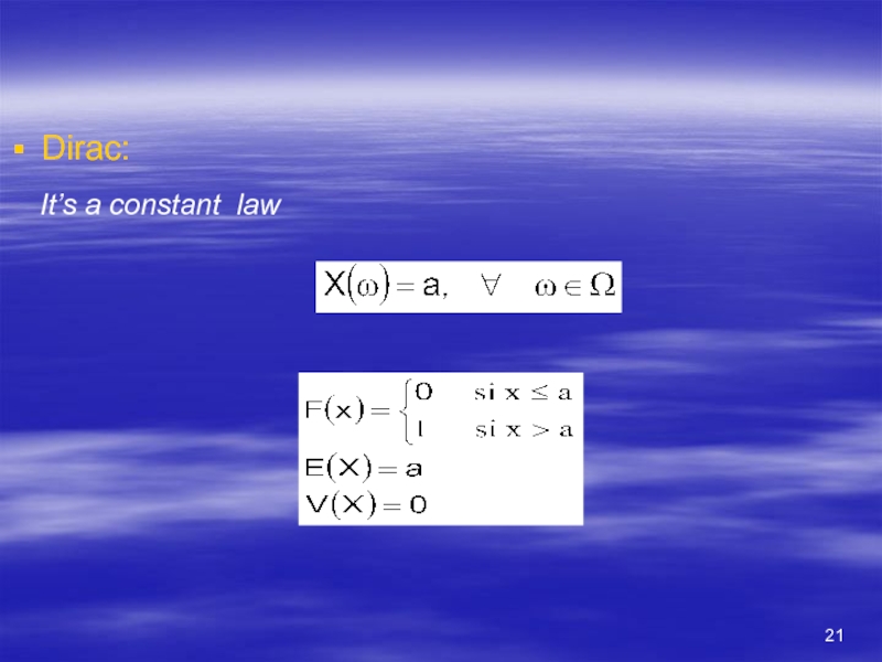
- 21. It’s a constant law Dirac:
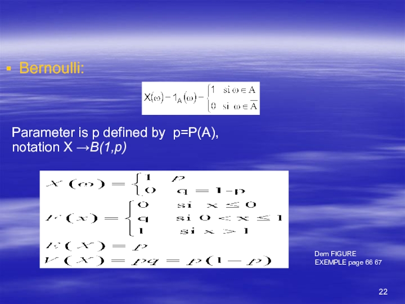
- 22. Bernoulli: Parameter is p defined by p=P(A),
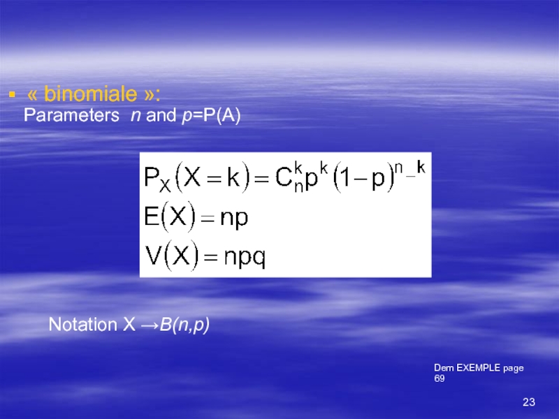
- 23. Parameters n and p=P(A) « binomiale »: Notation X →B(n,p) Dem EXEMPLE page 69
- 24. Parameters λ>0 « Poisson » : Notation X →P(λ) Dem EXEMPLE page 72 73 74
- 25. « Pascal »: Dem page 74 75 Parameter k
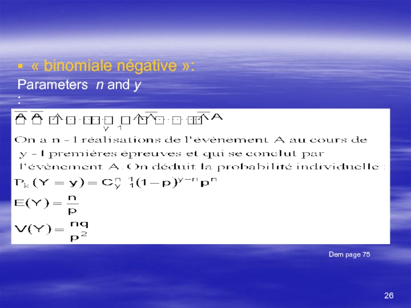
- 26. Parameters n and y : « binomiale négative »: Dem page 75
- 27. Continuous law Dem page 77 78
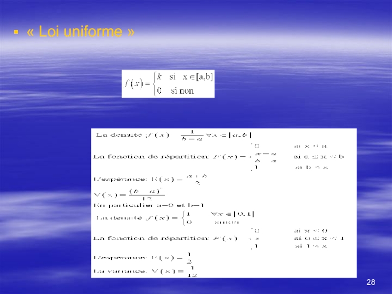
- 28. « Loi uniforme »
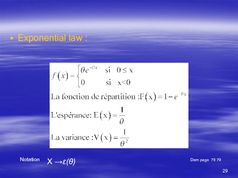
- 29. Exponential law : Notation X →ε(θ) Dem page 78 79
- 30. Laplace-Gauss: .Notation X →N(m, σ ) Dem page 79 80-83 Parameters m and σ
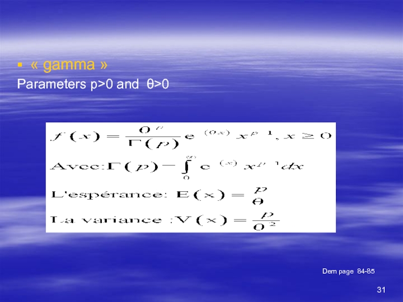
- 31. Parameters p>0 and θ>0 « gamma » Dem page 84-85
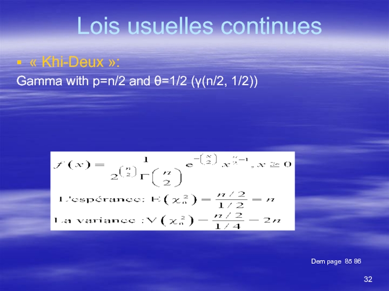
- 32. Lois usuelles continues Gamma with p=n/2 and θ=1/2 (γ(n/2, 1/2)) « Khi-Deux »: Dem page 85 86
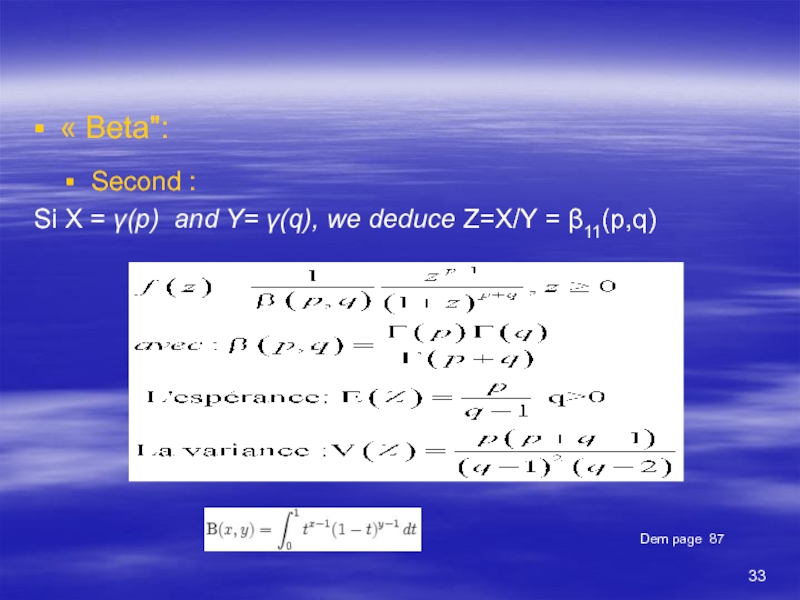
- 33. Si X = γ(p) and Y= γ(q),
- 34. « Beta »: First Dem page 88
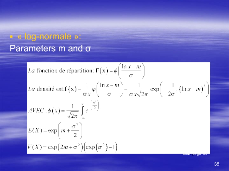
- 35. Parameters m and σ « log-normale »: Dem page 90
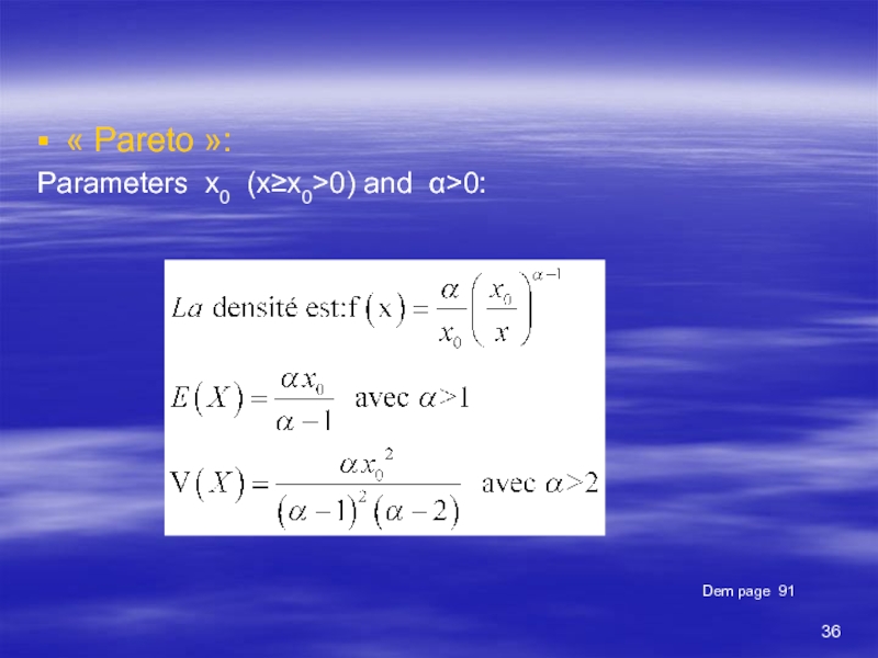
- 36. Parameters x0 (x≥x0>0) and α>0: « Pareto »: Dem page 91
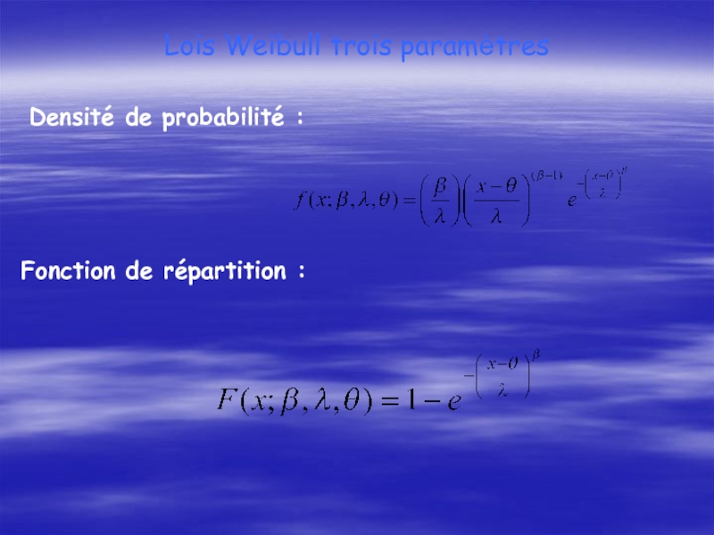
- 37. Lois Weibull trois paramètres Densité de probabilité : Fonction de répartition :
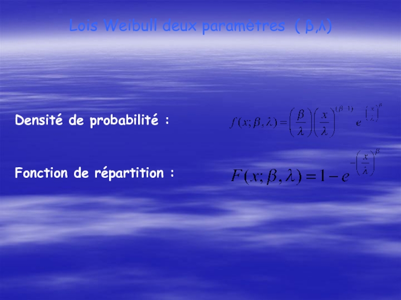
- 38. Lois Weibull deux paramètres ( β,λ) Densité
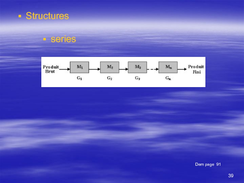
- 39. Structures Dem page 91 series
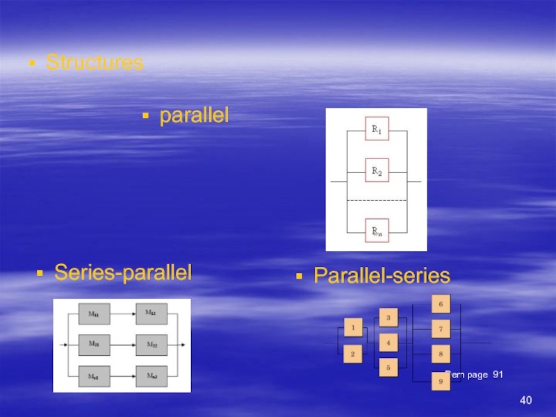
- 40. Structures Dem page 91 parallel Series-parallel Parallel-series
- 41. Complex Structures Bridge system Dem page 91 Theorem of Bays Exampl
- 42. Structures Dem page 91 series parallel Parallel-series Series-parallel
- 43. Structures Dem page 91 series parallel Parallel-series Series-parallel
- 44. Thank you for attention Dem page 91
Слайд 1Performance evaluation:
Point of view Reliability
System reliability
Sofiene Dellagi
University of Metz
Слайд 2Definition
It’s the probability of successful operation of a system or system
Motivation
Failures in airplanes, rockets or nuclear plants quickly become catastrophic; it is necessary to accurately predict the uptime of each of these systems. Currently, this study is the same time as the project construction
Слайд 3Definition and Notation
Reliability:
R(t) = Probability (S don’t fail on [0,t])
R(t) is
Availability:
Availability A (t) is the probability that the system S is not in default at time t. Note that in the case of non-repairable systems, the definition of A (t) is equivalent to the reliability : A(t) = Probability (S is not default at t )
Maintenability:
Maintainability M (t) :the probability that the system is repaired on the interval [0 t] knowing that he has failed at time t = 0 :
M(t)=Probability (S is repaired on [0 t]/ S is failed at t=0 )
This concept applies only to repairable systems
M(t) is a non decreasing function varying between 0 à 1 on [0, +∞ ⎡
Слайд 4Definitions et notations
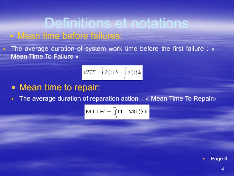
Mean time before failures:
Mean time to repair:
Page 4
The average
The average duration of reparation action : « Mean Time To Repair»
Слайд 5Definitions et notations
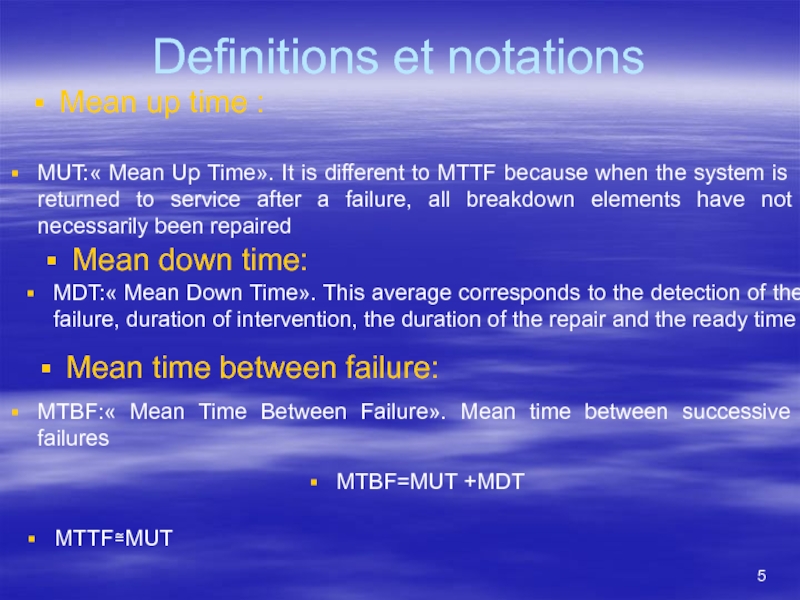
Mean up time :
MUT:« Mean Up Time». It is
Mean down time:
MDT:« Mean Down Time». This average corresponds to the detection of the failure, duration of intervention, the duration of the repair and the ready time
Mean time between failure:
MTBF:« Mean Time Between Failure». Mean time between successive failures
MTBF=MUT +MDT
MTTF≅MUT
Слайд 6stochastic Processes
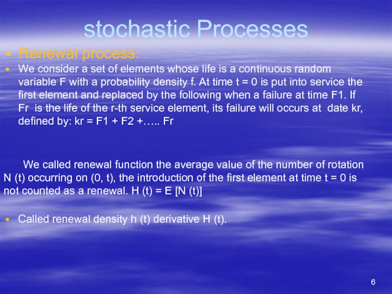
Renewal process:
We consider a set of elements whose life is
We called renewal function the average value of the number of rotation N (t) occurring on (0, t), the introduction of the first element at time t = 0 is not counted as a renewal. H (t) = E [N (t)]
Called renewal density h (t) derivative H (t).
Слайд 7stochastic Processes
We called variable renewal process a renewal process for which
We Called residual life Vt the random variable representing the remaining life of the item in service at time t
Page 25 26 27
Слайд 8Fondamental relations
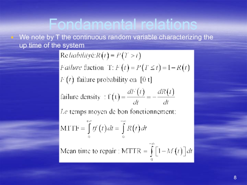
We note by T the continuous random variable characterizing the
Слайд 10Method of determination of the material failure law
« New material »
Experimentation
The Principe
Слайд 11Method of determination of the material failure law
« New material »
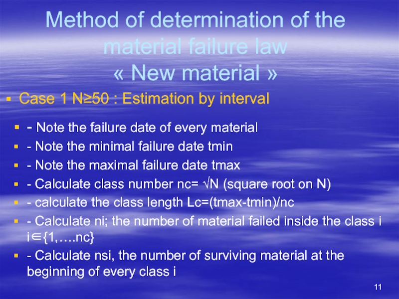
Case 1 N≥50
- Note the failure date of every material
- Note the minimal failure date tmin
- Note the maximal failure date tmax
- Calculate class number nc= √N (square root on N)
- calculate the class length Lc=(tmax-tmin)/nc
- Calculate ni; the number of material failed inside the class i i∈{1,….nc}
- Calculate nsi, the number of surviving material at the beginning of every class i
Слайд 12Method of determination of the material failure law
« New material »
Case 1 N≥50
Estimation of a failure law for every class
*probability density function for class i:
fi= ni/(N*Lc)
* Failure rate for class i:
λi= ni/(nsi*Lc)
* Reliability for class i
Ri= fi/ λi
* probability distribution function associated with the time to failure for class i
Fi=1-Ri
Слайд 13Method of determination of the material failure law
« New material »
Case 1 N≥50
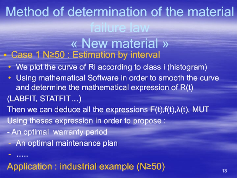
We plot the curve of Ri according to class i (histogram)
Using mathematical Software in order to smooth the curve and determine the mathematical expression of R(t)
(LABFIT, STATFIT…)
Then we can deduce all the expressions F(t),f(t),λ(t), MUT
Using theses expression in order to propose :
- An optimal warranty period
An optimal maintenance plan
…..
Application : industrial example (N≥50)
Слайд 14Method of determination of the material failure law
« New material »
Case 2 N
- Note the failure date of every material
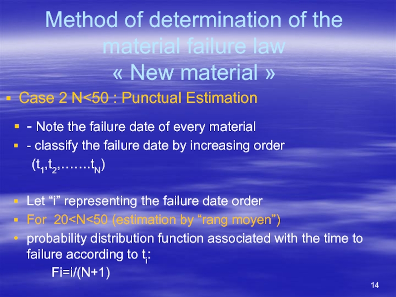
- classify the failure date by increasing order
(t1,t2,…….tN)
Let “i” representing the failure date order
For 20
Fi=i/(N+1)
Слайд 15Method of determination of the material failure law
« New material »
Case 2 N
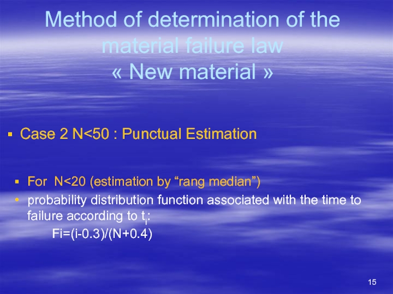
For N<20 (estimation by “rang median”)
probability distribution function associated with the time to failure according to ti:
Fi=(i-0.3)/(N+0.4)
Слайд 16Method of determination of the material failure law
« New material »
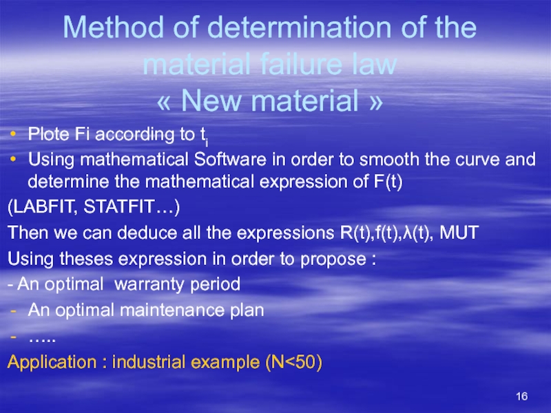
Plote Fi according
Using mathematical Software in order to smooth the curve and determine the mathematical expression of F(t)
(LABFIT, STATFIT…)
Then we can deduce all the expressions R(t),f(t),λ(t), MUT
Using theses expression in order to propose :
- An optimal warranty period
An optimal maintenance plan
…..
Application : industrial example (N<50)
Слайд 17Acceptance test for obtained law
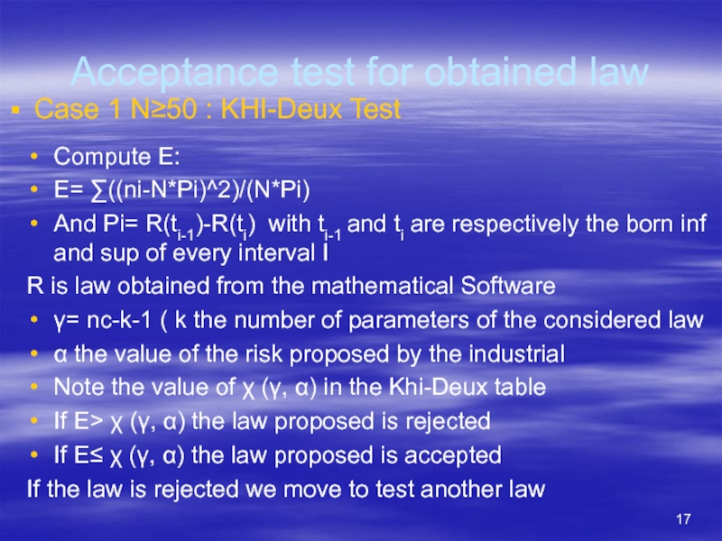
Case 1 N≥50 : KHI-Deux Test
Compute E:
E= ∑((ni-N*Pi)^2)/(N*Pi)
And Pi= R(ti-1)-R(ti) with ti-1 and ti are respectively the born inf and sup of every interval I
R is law obtained from the mathematical Software
γ= nc-k-1 ( k the number of parameters of the considered law
α the value of the risk proposed by the industrial
Note the value of χ (γ, α) in the Khi-Deux table
If E> χ (γ, α) the law proposed is rejected
If E≤ χ (γ, α) the law proposed is accepted
If the law is rejected we move to test another law
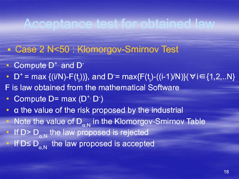
Слайд 18Acceptance test for obtained law
Case 2 N
D+ = max {(i/N)-F(ti))}, and D-= max{F(ti)-((i-1)/N)}(∀i∈{1,2,..N}
F is law obtained from the mathematical Software
Compute D= max (D+, D-)
α the value of the risk proposed by the industrial
Note the value of Dα,N in the Klomorgov-Smirnov Table
If D> Dα,N the law proposed is rejected
If D≤ Dα,N the law proposed is accepted

![Definition and NotationReliability:R(t) = Probability (S don’t fail on [0,t])R(t) is a non increasing function](/img/tmb/5/436173/88e17cce3926c8140945e17c120b90a9-800x.jpg)
