- Главная
- Разное
- Дизайн
- Бизнес и предпринимательство
- Аналитика
- Образование
- Развлечения
- Красота и здоровье
- Финансы
- Государство
- Путешествия
- Спорт
- Недвижимость
- Армия
- Графика
- Культурология
- Еда и кулинария
- Лингвистика
- Английский язык
- Астрономия
- Алгебра
- Биология
- География
- Детские презентации
- Информатика
- История
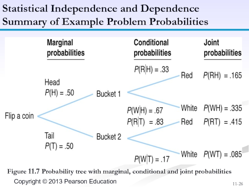
- Литература
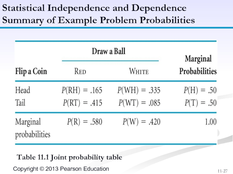
- Маркетинг
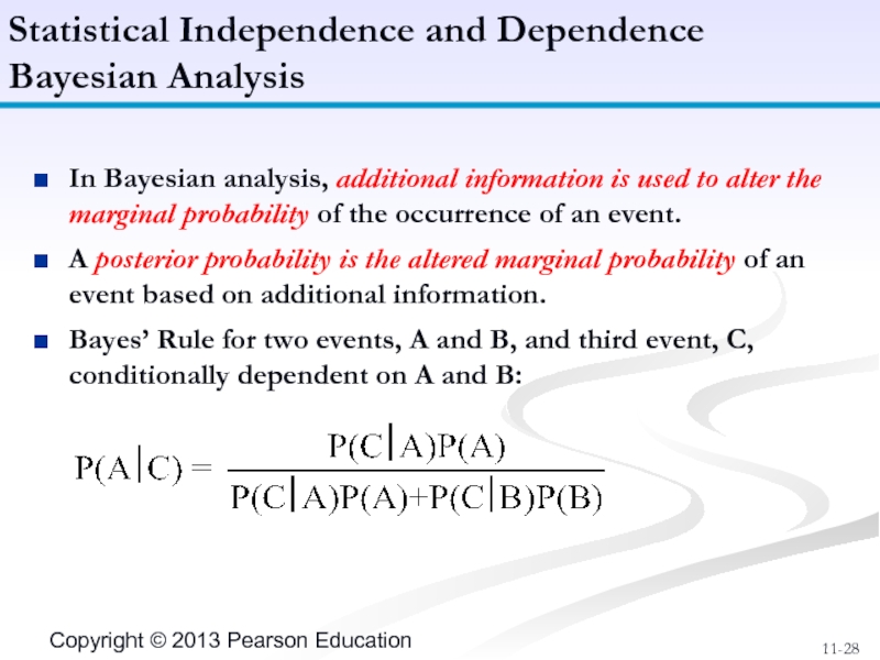
- Математика
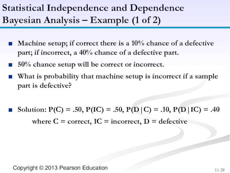
- Медицина
- Менеджмент
- Музыка
- МХК
- Немецкий язык
- ОБЖ
- Обществознание
- Окружающий мир
- Педагогика
- Русский язык
- Технология
- Физика
- Философия
- Химия
- Шаблоны, картинки для презентаций
- Экология
- Экономика
- Юриспруденция
Probabilistic Models. Chapter 11 презентация
Содержание
- 1. Probabilistic Models. Chapter 11
- 2. Types of Probability Fundamentals of Probability Statistical
- 3. Deterministic techniques assume that no uncertainty exists
- 4. Classical, or a priori (prior to the
- 5. Subjective probability is an estimate based on
- 6. An experiment is an activity that results
- 7. A frequency distribution is an organization of
- 8. State University, 3000 students, management science grades
- 9. A marginal probability is the probability of
- 10. Figure 11.1 Venn Diagram for Mutually
- 11. Probability that non-mutually exclusive events A and
- 12. Figure 11.2 Venn diagram for non–mutually exclusive
- 13. Can be developed by adding the probability
- 14. A succession of events that do not
- 15. For coin tossed three consecutive times
- 16. Properties of a Bernoulli Process: There
- 17. A binomial probability distribution function is used
- 18. Determine probability of getting exactly two tails
- 19. Microchip production; sample of four items per
- 20. Four microchips tested per batch; if two
- 21. Figure 11.4 Dependent events Statistical Independence and Dependence Dependent Events (1 of 2)
- 22. If the occurrence of one event affects
- 23. Unconditional: P(H) = .5; P(T) =
- 24. Conditional: P(R|H) =.33, P(W|H) =
- 25. Given two dependent events A and B:
- 26. Figure 11.7 Probability tree with marginal, conditional
- 27. Table 11.1 Joint probability table Statistical Independence and Dependence Summary of Example Problem Probabilities
- 28. In Bayesian analysis, additional information is used
- 29. Machine setup; if correct there is a
- 30. Posterior probabilities: Statistical Independence and Dependence Bayesian Analysis – Example (2 of 2)
- 31. When the values of variables occur in
- 32. Machines break down 0, 1, 2, 3,
- 33. The expected value of a random variable
- 34. Variance is a measure of the dispersion
- 35. Standard deviation is computed by taking the
- 36. A continuous random variable can take on
- 37. The normal distribution is a continuous probability
- 38. Mean weekly carpet sales of 4,200 yards,
- 39. - - Figure 11.9 The normal
- 40. The area or probability under a normal
- 41. The Normal Distribution Standard Normal Curve (2
- 42. Figure 11.11 Determination of the Z
- 43. Determine the probability that demand will be
- 44. The Normal Distribution Example (5 of 5)
- 45. The population mean and variance are for
- 46. The Normal Distribution Computing the Sample
- 47. Sample mean = 42,000/10 = 4,200 yd
- 48. It can never be simply assumed that
- 49. In the test, the actual number of
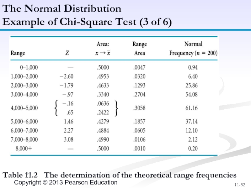
- 50. Armor Carpet Store example - assume sample
- 51. Figure 11.14 The theoretical normal distribution The
- 52. Table 11.2 The determination of the
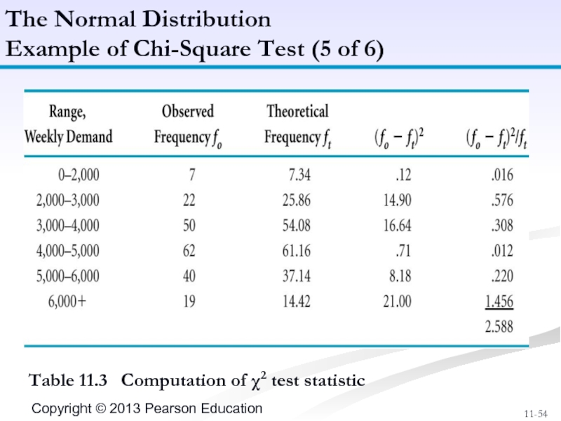
- 53. The Normal Distribution Example of Chi-Square Test
- 54. Table 11.3 Computation of χ2 test
- 55. χ2k-p-1 = Σ(fo - ft)2/10 = 2.588
- 56. Exhibit 11.1 Statistical Analysis with Excel (1
- 57. Statistical Analysis with Excel (2 of 2)
- 58. Radcliff Chemical Company and Arsenal. Annual number
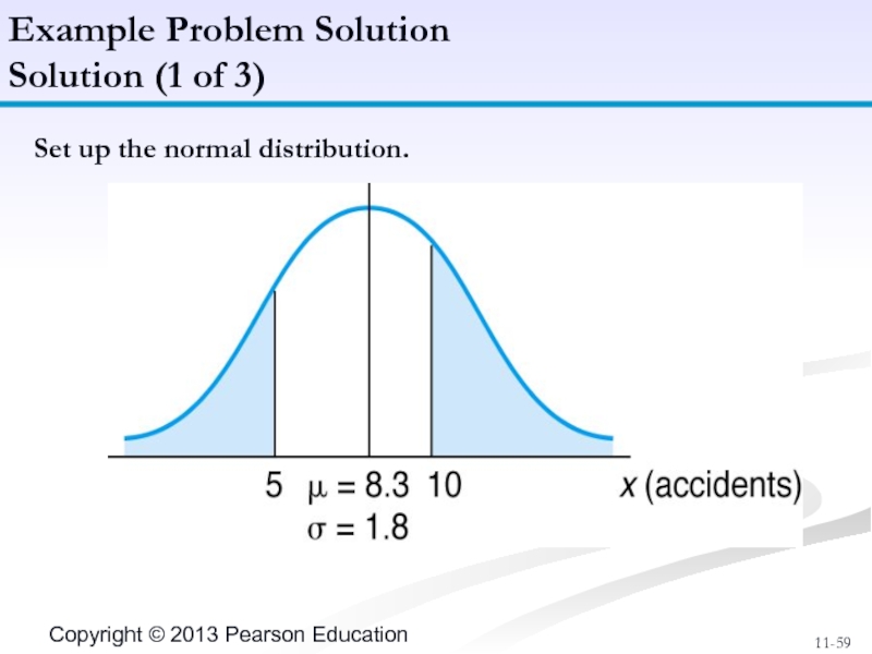
- 59. Set up the normal distribution. Example Problem Solution Solution (1 of 3)
- 60. Solve Part 1: P(x ≤ 5 accidents)
- 61. Solve Part 2: P(x ≥ 12
- 62. All rights reserved. No part of this
Слайд 2Types of Probability
Fundamentals of Probability
Statistical Independence and Dependence
Expected Value
The Normal Distribution
Chapter
Слайд 3Deterministic techniques assume that no uncertainty exists in model parameters. Chapters
Probabilistic techniques include uncertainty and assume that there can be more than one model solution.
There is some doubt about which outcome will occur.
Solutions may be in the form of averages.
Overview
Слайд 4Classical, or a priori (prior to the occurrence), probability is an
Objective probabilities that are stated after the outcomes of an event have been observed are relative frequencies, based on observation of past occurrences.
Relative frequency is the more widely used definition of objective probability.
Types of Probability
Objective Probability
Слайд 5Subjective probability is an estimate based on personal belief, experience, or
It is often the only means available for making probabilistic estimates.
Frequently used in making business decisions.
Different people often arrive at different subjective probabilities.
Objective probabilities are used in this text unless otherwise indicated.
Types of Probability
Subjective Probability
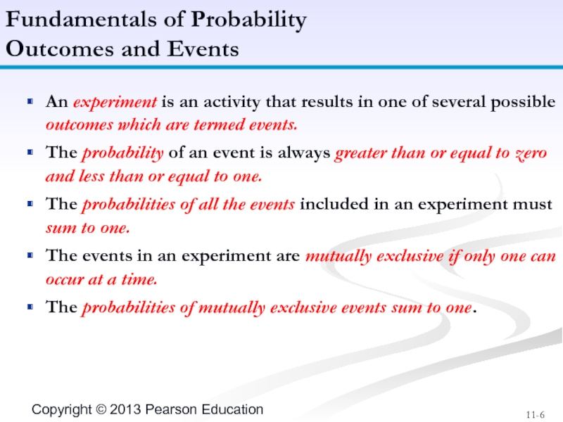
Слайд 6An experiment is an activity that results in one of several
The probability of an event is always greater than or equal to zero and less than or equal to one.
The probabilities of all the events included in an experiment must sum to one.
The events in an experiment are mutually exclusive if only one can occur at a time.
The probabilities of mutually exclusive events sum to one.
Fundamentals of Probability
Outcomes and Events
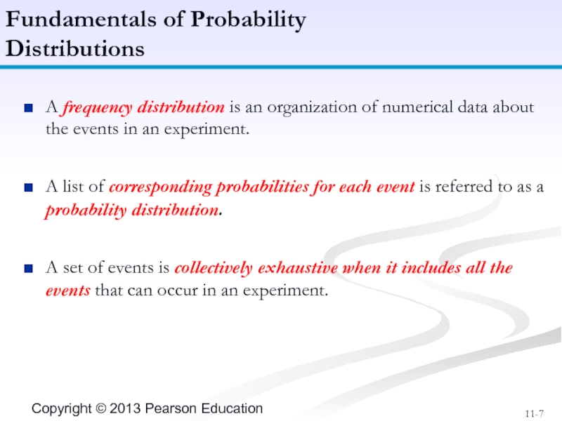
Слайд 7A frequency distribution is an organization of numerical data about the
A list of corresponding probabilities for each event is referred to as a probability distribution.
A set of events is collectively exhaustive when it includes all the events that can occur in an experiment.
Fundamentals of Probability
Distributions
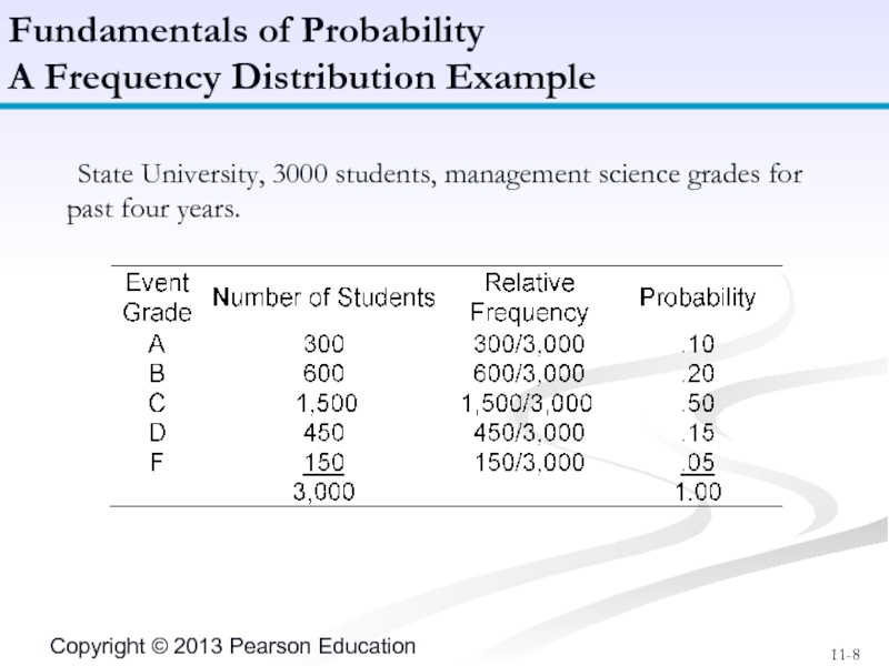
Слайд 8 State University, 3000 students, management science grades for past four years.
Fundamentals
A Frequency Distribution Example
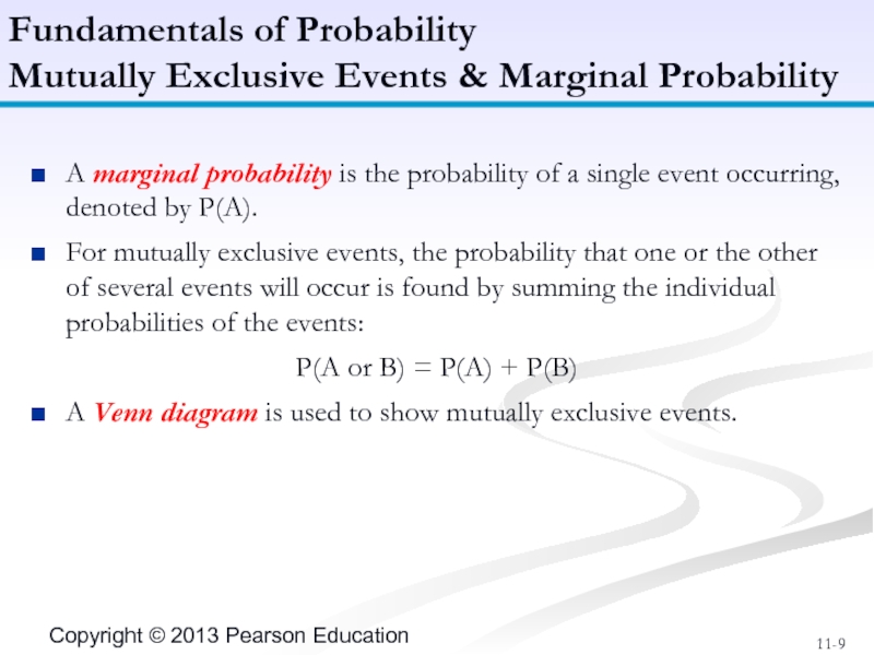
Слайд 9A marginal probability is the probability of a single event occurring,
For mutually exclusive events, the probability that one or the other of several events will occur is found by summing the individual probabilities of the events:
P(A or B) = P(A) + P(B)
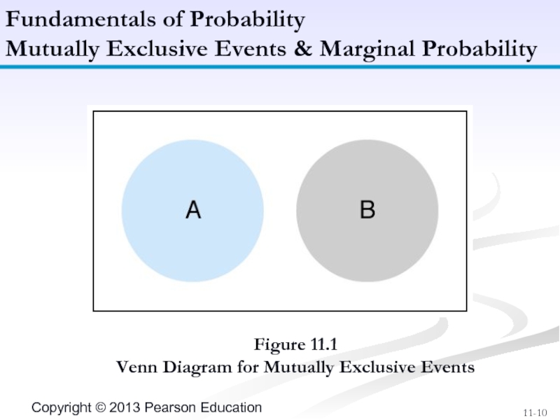
A Venn diagram is used to show mutually exclusive events.
Fundamentals of Probability
Mutually Exclusive Events & Marginal Probability
Слайд 10
Figure 11.1
Venn Diagram for Mutually Exclusive Events
Fundamentals of Probability
Mutually Exclusive Events
Слайд 11Probability that non-mutually exclusive events A and B or both will
P(A or B) = P(A) + P(B) - P(AB)
A joint probability, P(AB), is the probability that two or more events that are not mutually exclusive can occur simultaneously.
Fundamentals of Probability
Non-Mutually Exclusive Events & Joint Probability
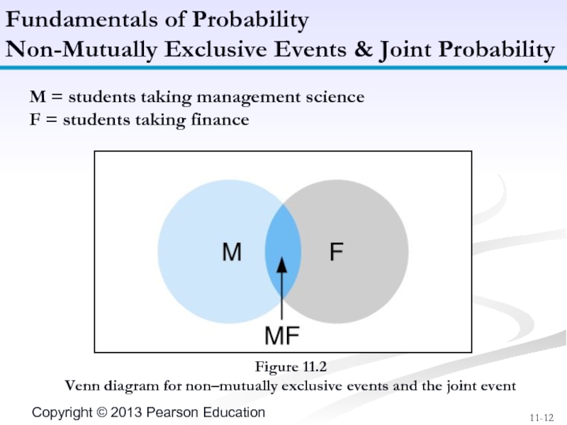
Слайд 12Figure 11.2
Venn diagram for non–mutually exclusive events and the joint event
Fundamentals
Non-Mutually Exclusive Events & Joint Probability
M = students taking management science
F = students taking finance
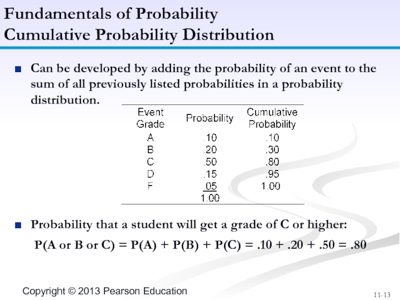
Слайд 13Can be developed by adding the probability of an event to
Probability that a student will get a grade of C or higher:
P(A or B or C) = P(A) + P(B) + P(C) = .10 + .20 + .50 = .80
Fundamentals of Probability
Cumulative Probability Distribution
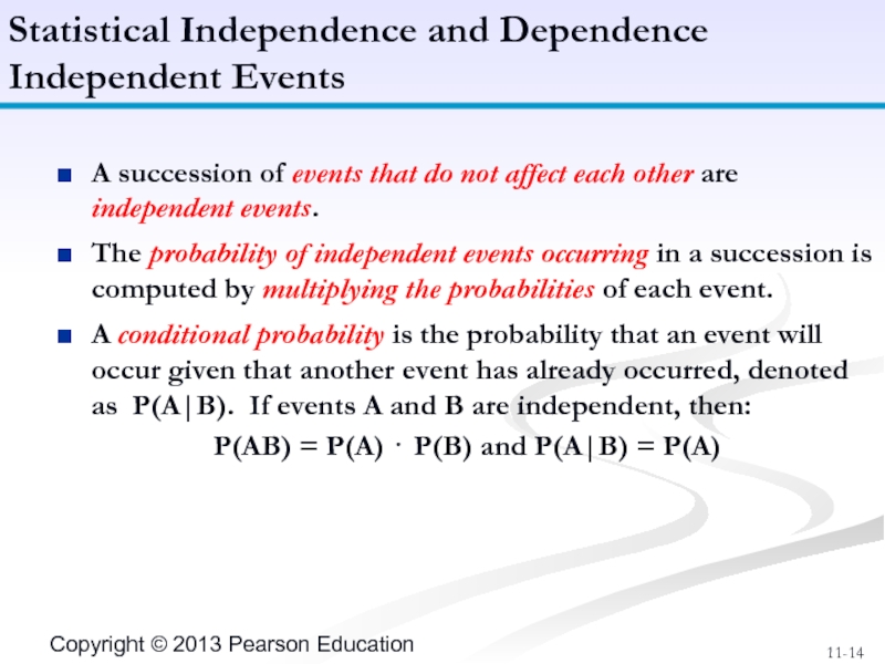
Слайд 14A succession of events that do not affect each other are
The probability of independent events occurring in a succession is computed by multiplying the probabilities of each event.
A conditional probability is the probability that an event will occur given that another event has already occurred, denoted as P(A|B). If events A and B are independent, then:
P(AB) = P(A) ⋅ P(B) and P(A|B) = P(A)
Statistical Independence and Dependence
Independent Events
Слайд 15
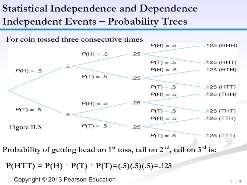
For coin tossed three consecutive times
Figure 11.3
Statistical Independence and Dependence
Independent Events
Probability of getting head on 1st toss, tail on 2nd, tail on 3rd is:
P(HTT) = P(H) ⋅ P(T) ⋅ P(T)=(.5)(.5)(.5)=.125
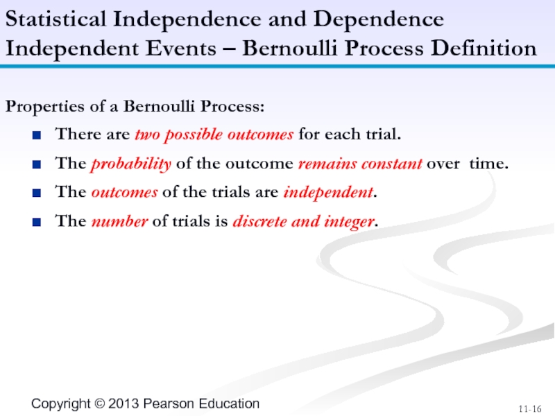
Слайд 16Properties of a Bernoulli Process:
There are two possible outcomes for
The probability of the outcome remains constant over time.
The outcomes of the trials are independent.
The number of trials is discrete and integer.
Statistical Independence and Dependence
Independent Events – Bernoulli Process Definition
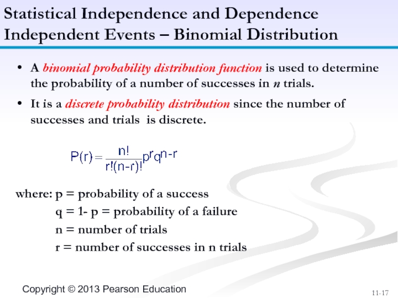
Слайд 17A binomial probability distribution function is used to determine the probability
It is a discrete probability distribution since the number of successes and trials is discrete.
where: p = probability of a success
q = 1- p = probability of a failure
n = number of trials
r = number of successes in n trials
Statistical Independence and Dependence
Independent Events – Binomial Distribution
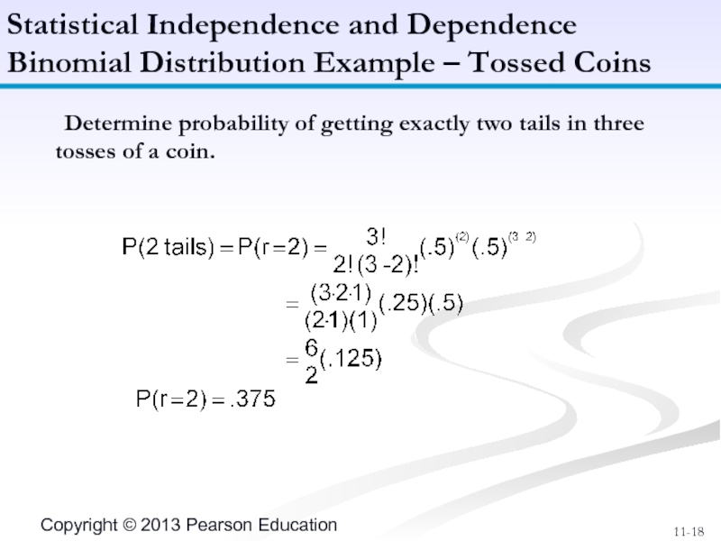
Слайд 18 Determine probability of getting exactly two tails in three tosses of
Statistical Independence and Dependence
Binomial Distribution Example – Tossed Coins
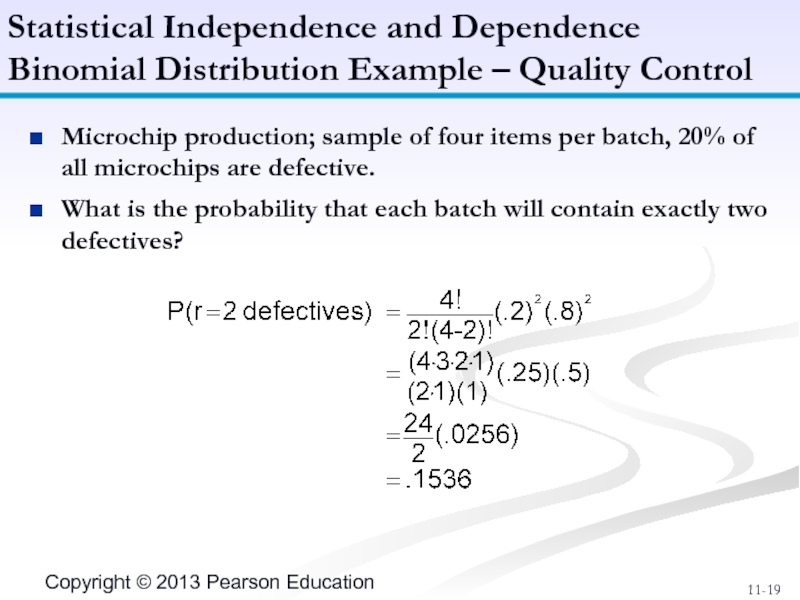
Слайд 19Microchip production; sample of four items per batch, 20% of all
What is the probability that each batch will contain exactly two defectives?
Statistical Independence and Dependence
Binomial Distribution Example – Quality Control
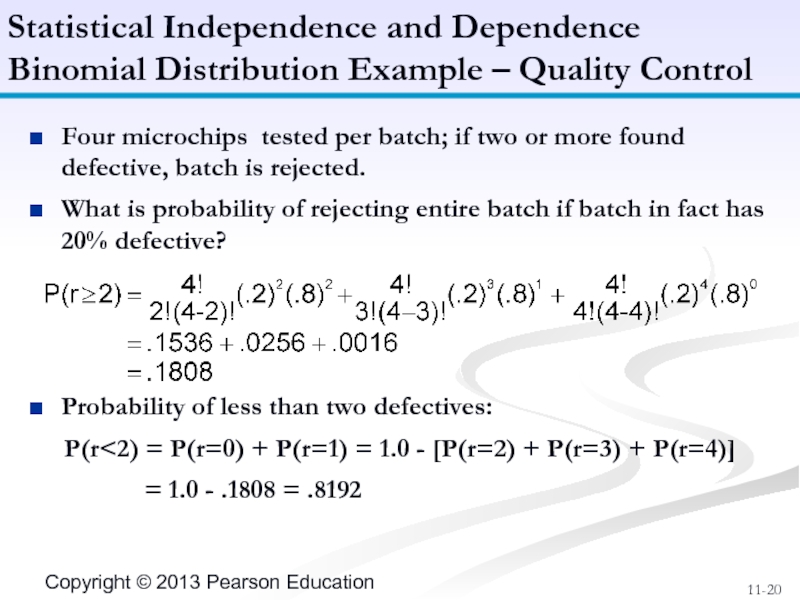
Слайд 20Four microchips tested per batch; if two or more found defective,
What is probability of rejecting entire batch if batch in fact has 20% defective?
Probability of less than two defectives:
P(r<2) = P(r=0) + P(r=1) = 1.0 - [P(r=2) + P(r=3) + P(r=4)]
= 1.0 - .1808 = .8192
Statistical Independence and Dependence
Binomial Distribution Example – Quality Control
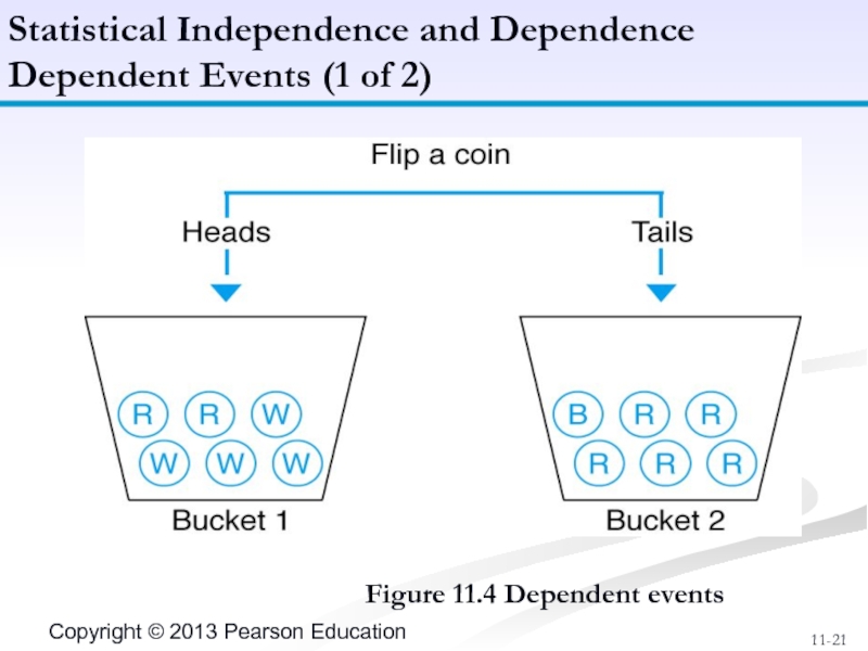
Слайд 21Figure 11.4 Dependent events
Statistical Independence and Dependence
Dependent Events (1 of 2)
Слайд 22If the occurrence of one event affects the probability of the
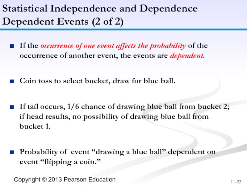
Coin toss to select bucket, draw for blue ball.
If tail occurs, 1/6 chance of drawing blue ball from bucket 2; if head results, no possibility of drawing blue ball from bucket 1.
Probability of event “drawing a blue ball” dependent on event “flipping a coin.”
Statistical Independence and Dependence
Dependent Events (2 of 2)
Слайд 23
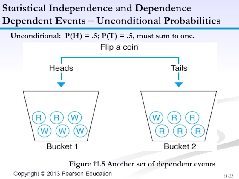
Unconditional: P(H) = .5; P(T) = .5, must sum to one.
Figure
Statistical Independence and Dependence
Dependent Events – Unconditional Probabilities
Слайд 24
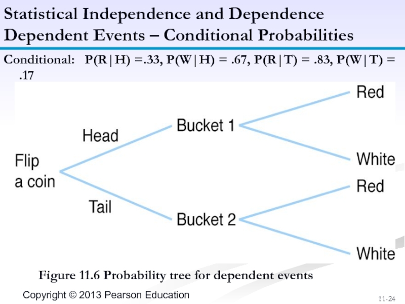
Conditional: P(R|H) =.33, P(W|H) = .67, P(R|T) = .83, P(W|T)
Statistical Independence and Dependence
Dependent Events – Conditional Probabilities
Figure 11.6 Probability tree for dependent events
Слайд 25Given two dependent events A and B:
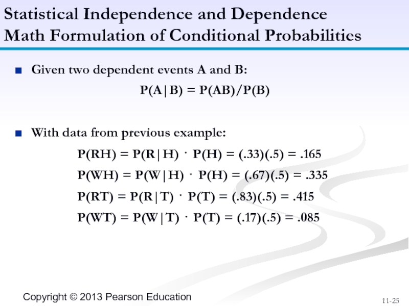
P(A|B) = P(AB)/P(B)
With data from
P(RH) = P(R|H) ⋅ P(H) = (.33)(.5) = .165
P(WH) = P(W|H) ⋅ P(H) = (.67)(.5) = .335
P(RT) = P(R|T) ⋅ P(T) = (.83)(.5) = .415
P(WT) = P(W|T) ⋅ P(T) = (.17)(.5) = .085
Statistical Independence and Dependence
Math Formulation of Conditional Probabilities
Слайд 26Figure 11.7 Probability tree with marginal, conditional and joint probabilities
Statistical Independence
Summary of Example Problem Probabilities
Слайд 27Table 11.1 Joint probability table
Statistical Independence and Dependence
Summary of Example Problem
Слайд 28In Bayesian analysis, additional information is used to alter the marginal
A posterior probability is the altered marginal probability of an event based on additional information.
Bayes’ Rule for two events, A and B, and third event, C, conditionally dependent on A and B:
Statistical Independence and Dependence
Bayesian Analysis
Слайд 29Machine setup; if correct there is a 10% chance of a
50% chance setup will be correct or incorrect.
What is probability that machine setup is incorrect if a sample part is defective?
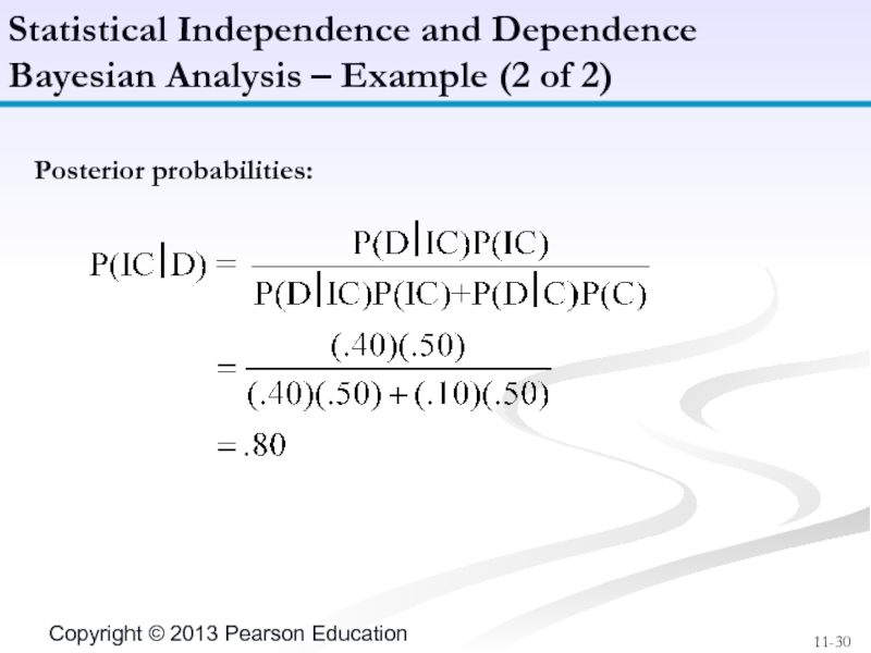
Solution: P(C) = .50, P(IC) = .50, P(D|C) = .10, P(D|IC) = .40
where C = correct, IC = incorrect, D = defective
Statistical Independence and Dependence
Bayesian Analysis – Example (1 of 2)
Слайд 30Posterior probabilities:
Statistical Independence and Dependence
Bayesian Analysis – Example (2 of 2)
Слайд 31When the values of variables occur in no particular order or
Random variables are represented symbolically by a letter x, y, z, etc.
Although exact values of random variables are not known prior to events, it is possible to assign a probability to the occurrence of possible values.
Expected Value
Random Variables
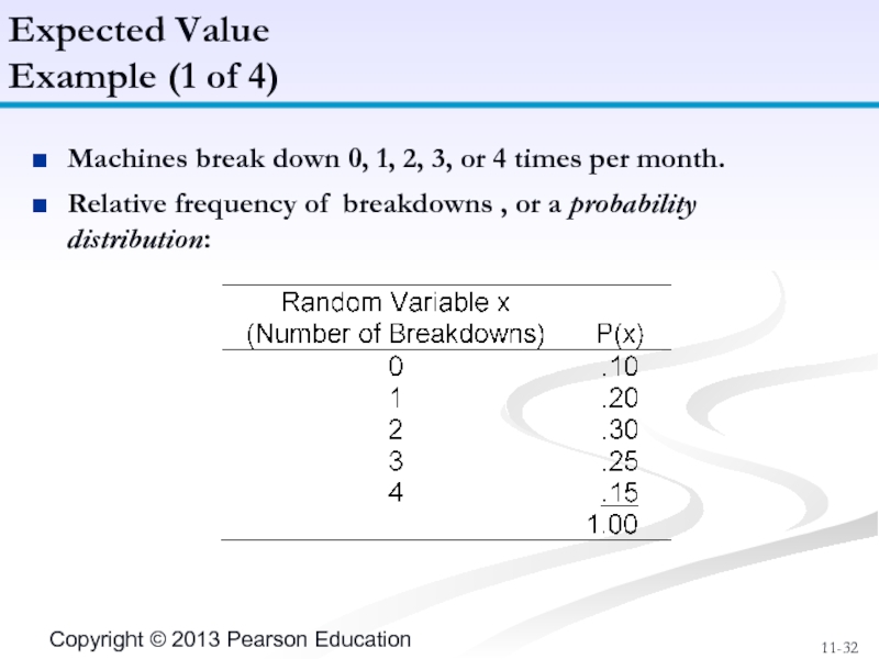
Слайд 32Machines break down 0, 1, 2, 3, or 4 times per
Relative frequency of breakdowns , or a probability distribution:
Expected Value
Example (1 of 4)
Слайд 33The expected value of a random variable is computed by multiplying
The expected value is the weighted average, or mean, of the probability distribution of the random variable.
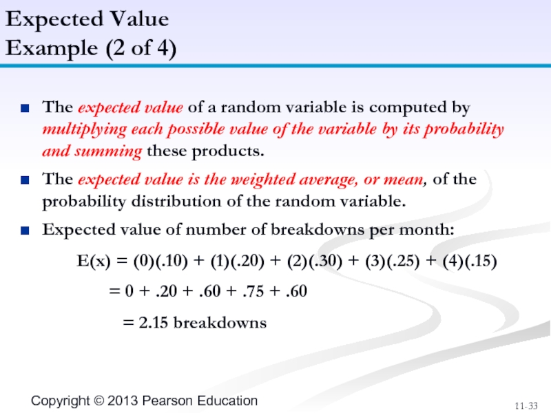
Expected value of number of breakdowns per month:
E(x) = (0)(.10) + (1)(.20) + (2)(.30) + (3)(.25) + (4)(.15)
= 0 + .20 + .60 + .75 + .60
= 2.15 breakdowns
Expected Value
Example (2 of 4)
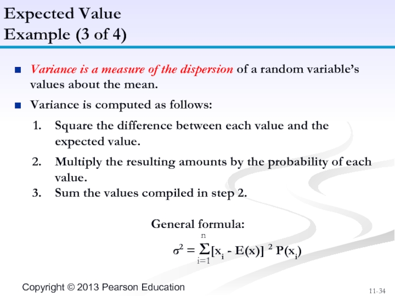
Слайд 34Variance is a measure of the dispersion of a random variable’s
Variance is computed as follows:
Square the difference between each value and the expected value.
Multiply the resulting amounts by the probability of each value.
Sum the values compiled in step 2.
General formula:
σ2 = Σ[xi - E(x)] 2 P(xi)
Expected Value
Example (3 of 4)
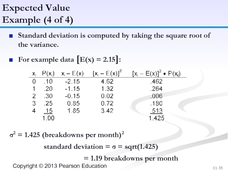
Слайд 35Standard deviation is computed by taking the square root of the
For example data [E(x) = 2.15]:
σ2 = 1.425 (breakdowns per month)2
standard deviation = σ = sqrt(1.425)
= 1.19 breakdowns per month
Expected Value
Example (4 of 4)
Слайд 36A continuous random variable can take on an infinite number of
Continuous random variables have values that are not specifically countable and are often fractional.
Cannot assign a unique probability to each value of a continuous random variable.
In a continuous probability distribution the probability refers to a value of the random variable being within some range.
The Normal Distribution
Continuous Random Variables
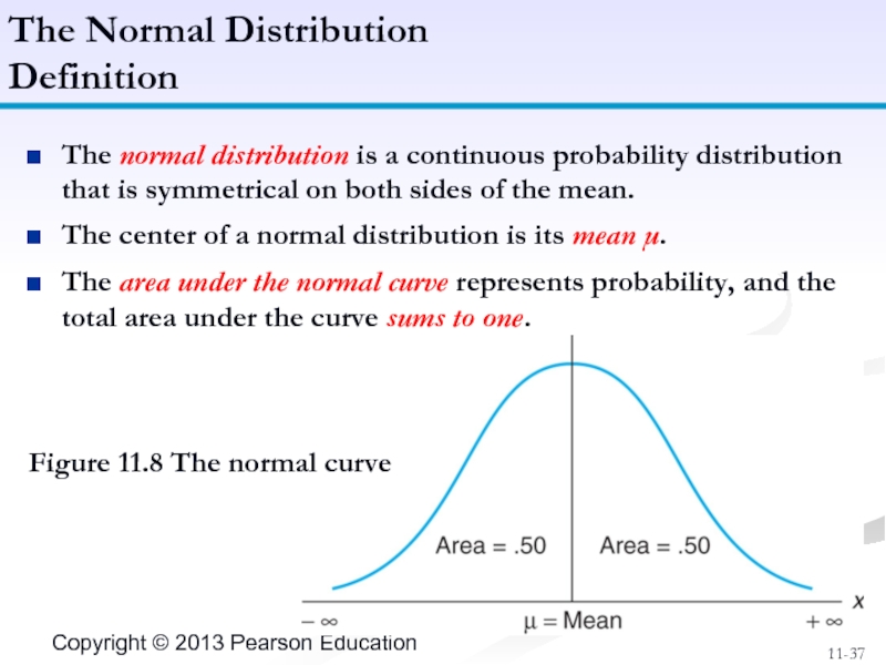
Слайд 37The normal distribution is a continuous probability distribution that is symmetrical
The center of a normal distribution is its mean μ.
The area under the normal curve represents probability, and the total area under the curve sums to one.
The Normal Distribution
Definition
Figure 11.8 The normal curve
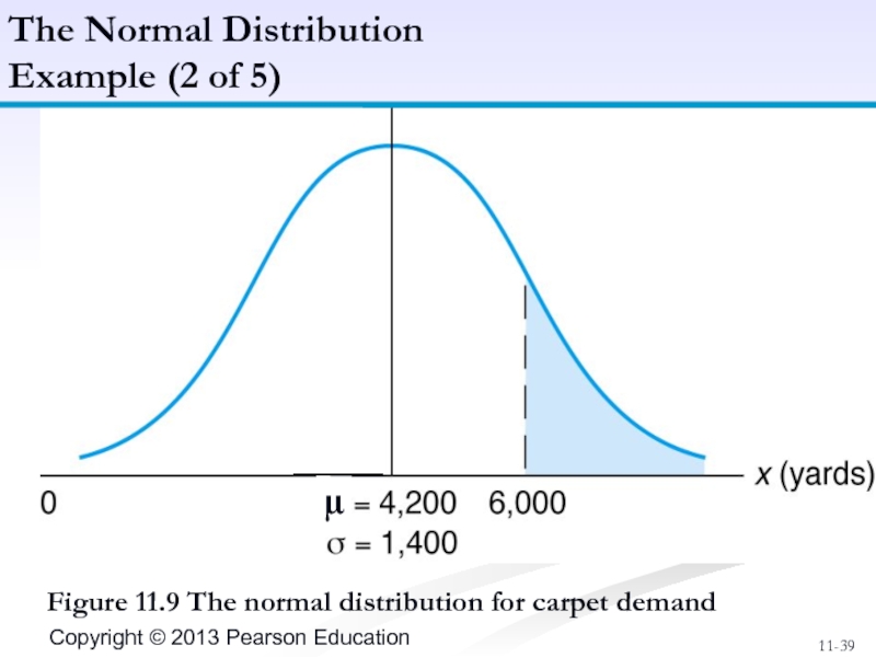
Слайд 38Mean weekly carpet sales of 4,200 yards, with a standard deviation
What is the probability of sales exceeding 6,000 yards?
μ = 4,200 yd; σ = 1,400 yd; probability that number of yards of carpet will be equal to or greater than 6,000 expressed as: P(x≥6,000).
The Normal Distribution
Example (1 of 5)
Слайд 39-
-
Figure 11.9 The normal distribution for carpet demand
The Normal Distribution
Example (2
P(x≥6,000)
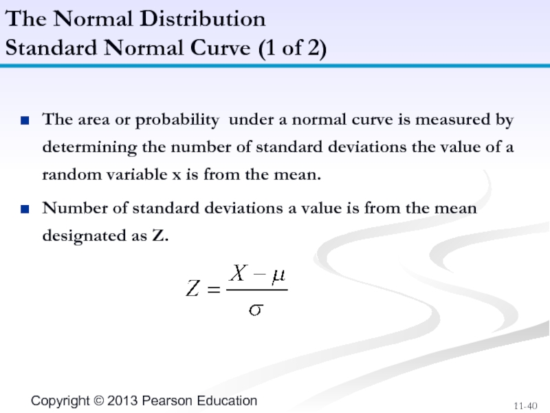
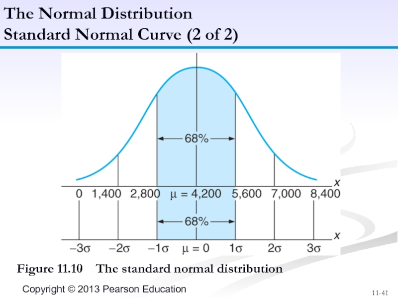
Слайд 40The area or probability under a normal curve is measured by
Number of standard deviations a value is from the mean designated as Z.
The Normal Distribution
Standard Normal Curve (1 of 2)
Слайд 41The Normal Distribution
Standard Normal Curve (2 of 2)
Figure 11.10 The
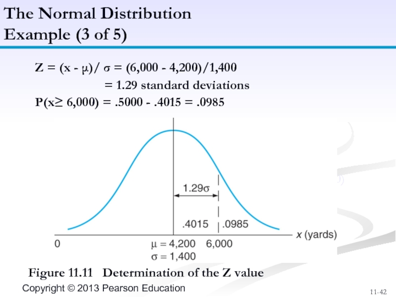
Слайд 42Figure 11.11 Determination of the Z value
The Normal Distribution
Example (3
Z = (x - μ)/ σ = (6,000 - 4,200)/1,400
= 1.29 standard deviations
P(x≥ 6,000) = .5000 - .4015 = .0985
P(x≥6,000)
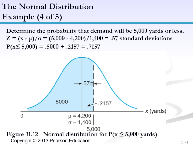
Слайд 43Determine the probability that demand will be 5,000 yards or less.
Z
P(x≤ 5,000) = .5000 + .2157 = .7157
The Normal Distribution
Example (4 of 5)
Figure 11.12 Normal distribution for P(x ≤ 5,000 yards)
Слайд 44The Normal Distribution
Example (5 of 5)
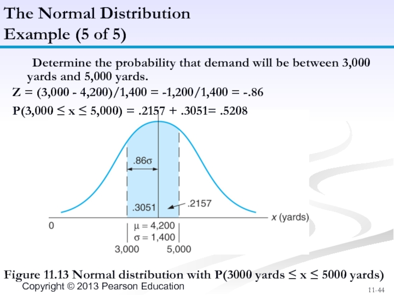
Figure 11.13 Normal distribution with P(3000
Determine the probability that demand will be between 3,000 yards and 5,000 yards.
Z = (3,000 - 4,200)/1,400 = -1,200/1,400 = -.86
P(3,000 ≤ x ≤ 5,000) = .2157 + .3051= .5208
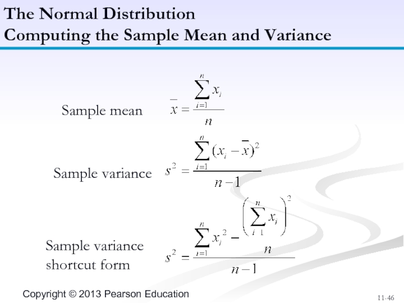
Слайд 45The population mean and variance are for the entire set of
The sample mean and variance are derived from a subset of the population data and are used to make inferences about the population.
The Normal Distribution
Sample Mean and Variance
Слайд 46
The Normal Distribution
Computing the Sample Mean and Variance
Sample mean
Sample variance
Sample variance
Слайд 47Sample mean = 42,000/10 = 4,200 yd
Sample variance = [(190,060,000) -
= 1,517,777
Sample std. dev. = sqrt(1,517,777)
= 1,232 yd
The Normal Distribution
Example Problem Revisited
Слайд 48It can never be simply assumed that data are normally distributed.
The
The chi-square test compares an observed frequency distribution with a theoretical frequency distribution (testing the goodness-of-fit).
The Normal Distribution
Chi-Square Test for Normality (1 of 2)
Слайд 49In the test, the actual number of frequencies in each range
A chi-square statistic is then calculated and compared to a number, called a critical value, from a chi-square table.
If the test statistic is greater than the critical value, the distribution does not follow the distribution being tested; if it is less, the distribution fits.
The chi-square test is a form of hypothesis testing.
The Normal Distribution
Chi-Square Test for Normality (2 of 2)
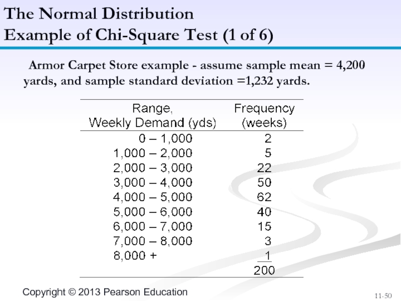
Слайд 50 Armor Carpet Store example - assume sample mean = 4,200 yards,
The Normal Distribution
Example of Chi-Square Test (1 of 6)
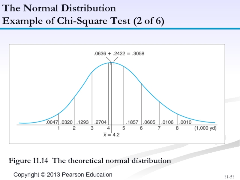
Слайд 51Figure 11.14 The theoretical normal distribution
The Normal Distribution
Example of Chi-Square Test
Слайд 52Table 11.2 The determination of the theoretical range frequencies
The Normal
Example of Chi-Square Test (3 of 6)
Слайд 53The Normal Distribution
Example of Chi-Square Test (4 of 6)
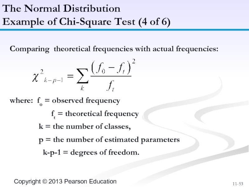
Comparing theoretical frequencies
where: fo = observed frequency
ft = theoretical frequency
k = the number of classes,
p = the number of estimated parameters
k-p-1 = degrees of freedom.
Слайд 54Table 11.3 Computation of χ2 test statistic
The Normal Distribution
Example
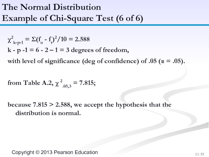
Слайд 55χ2k-p-1 = Σ(fo - ft)2/10 = 2.588
k - p -1 =
with level of significance (deg of confidence) of .05 (α = .05).
from Table A.2, χ 2.05,3 = 7.815;
because 7.815 > 2.588, we accept the hypothesis that the distribution is normal.
The Normal Distribution
Example of Chi-Square Test (6 of 6)
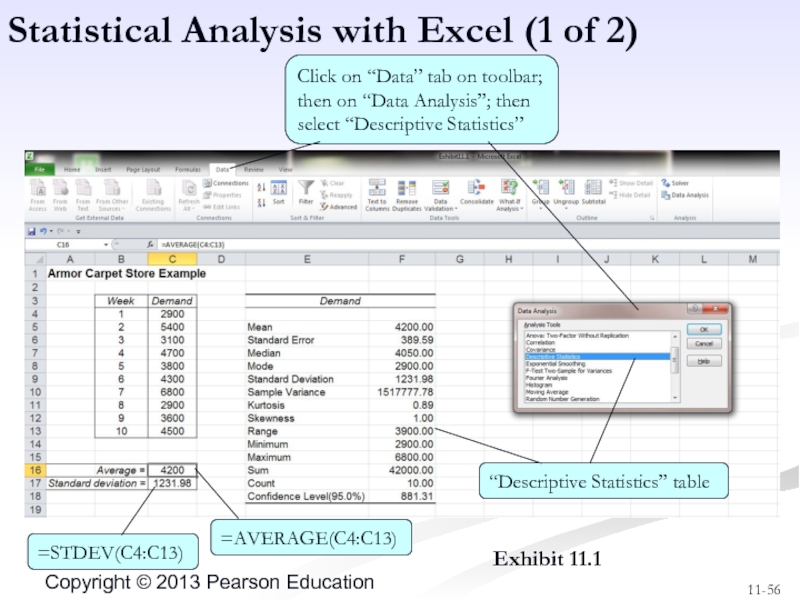
Слайд 56Exhibit 11.1
Statistical Analysis with Excel (1 of 2)
Click on “Data” tab
“Descriptive Statistics” table
=AVERAGE(C4:C13)
=STDEV(C4:C13)
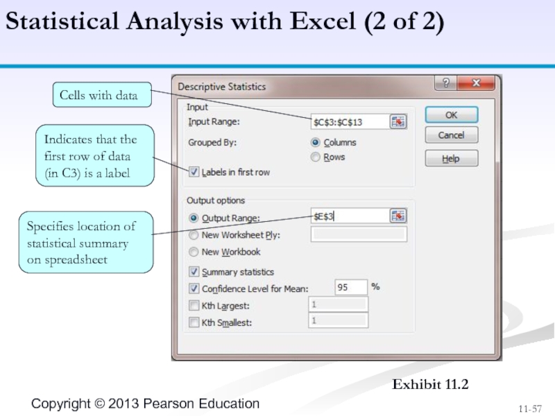
Слайд 57Statistical Analysis with Excel (2 of 2)
Exhibit 11.2
Cells with data
Indicates that
Specifies location of statistical summary on spreadsheet
Слайд 58Radcliff Chemical Company and Arsenal.
Annual number of accidents is normally distributed
What is the probability that the company will have fewer than five accidents next year? More than ten?
The government will fine the company $200,000 if the number of accidents exceeds 12 in a one-year period. What average annual fine can the company expect?
Example Problem Solution
Data
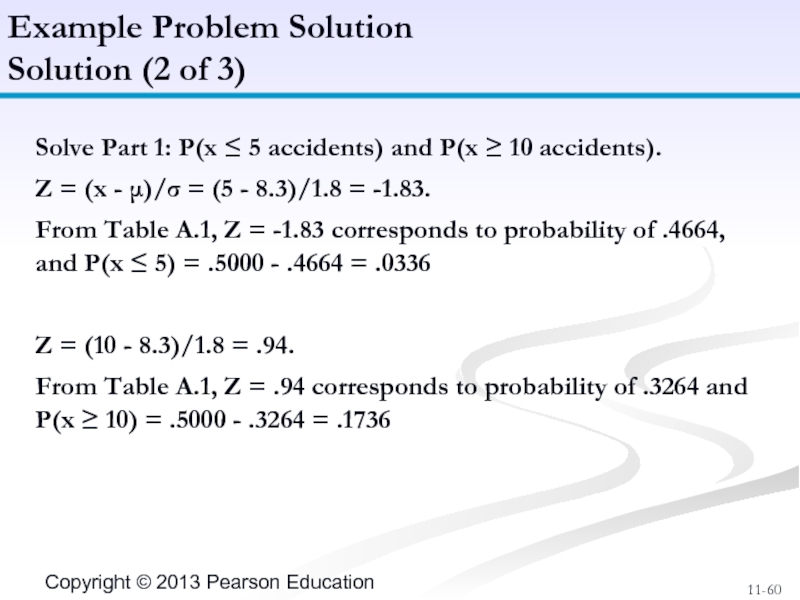
Слайд 60Solve Part 1: P(x ≤ 5 accidents) and P(x ≥ 10
Z = (x - μ)/σ = (5 - 8.3)/1.8 = -1.83.
From Table A.1, Z = -1.83 corresponds to probability of .4664, and P(x ≤ 5) = .5000 - .4664 = .0336
Z = (10 - 8.3)/1.8 = .94.
From Table A.1, Z = .94 corresponds to probability of .3264 and P(x ≥ 10) = .5000 - .3264 = .1736
Example Problem Solution
Solution (2 of 3)
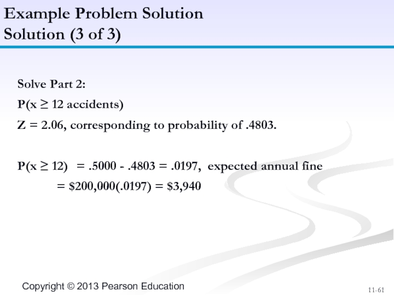
Слайд 61Solve Part 2:
P(x ≥ 12 accidents)
Z = 2.06, corresponding
P(x ≥ 12) = .5000 - .4803 = .0197, expected annual fine
= $200,000(.0197) = $3,940
Example Problem Solution
Solution (3 of 3)
Слайд 62All rights reserved. No part of this publication may be reproduced,
Printed in the United States of America.
![Sample mean = 42,000/10 = 4,200 ydSample variance = [(190,060,000) - (1,764,000,000/10)]/9 = 1,517,777Sample](/img/tmb/1/29697/72a5f9a11abd9d8bde4d11903e6cfe47-800x.jpg)
