Many slides borrowed
from Steve Seitz
- Главная
- Разное
- Дизайн
- Бизнес и предпринимательство
- Аналитика
- Образование
- Развлечения
- Красота и здоровье
- Финансы
- Государство
- Путешествия
- Спорт
- Недвижимость
- Армия
- Графика
- Культурология
- Еда и кулинария
- Лингвистика
- Английский язык
- Астрономия
- Алгебра
- Биология
- География
- Детские презентации
- Информатика
- История
- Литература
- Маркетинг
- Математика
- Медицина
- Менеджмент
- Музыка
- МХК
- Немецкий язык
- ОБЖ
- Обществознание
- Окружающий мир
- Педагогика
- Русский язык
- Технология
- Физика
- Философия
- Химия
- Шаблоны, картинки для презентаций
- Экология
- Экономика
- Юриспруденция
The Frequency Domain презентация
Содержание
- 1. The Frequency Domain
- 2. Salvador Dali, “Gala Contemplating the
- 5. A nice set of basis This
- 6. Jean Baptiste Joseph Fourier (1768-1830) had crazy
- 7. A sum of sines Our building block:
- 8. Fourier Transform We want to understand the
- 9. Time and Frequency example : g(t) = sin(2pf t) + (1/3)sin(2p(3f) t)
- 10. Time and Frequency example : g(t) = sin(2pf t) + (1/3)sin(2p(3f) t) = +
- 11. Frequency Spectra example : g(t) = sin(2pf t) + (1/3)sin(2p(3f) t) = +
- 12. Frequency Spectra Usually, frequency is more interesting than the phase
- 13. = + = Frequency Spectra
- 14. = + = Frequency Spectra
- 15. = + = Frequency Spectra
- 16. = + = Frequency Spectra
- 17. = + = Frequency Spectra
- 18. = Frequency Spectra
- 19. Frequency Spectra
- 20. FT: Just a change of basis .
- 21. IFT: Just a change of basis .
- 22. Finally: Scary Math
- 23. Finally: Scary Math …not really scary: is
- 24. Extension to 2D in Matlab, check out: imagesc(log(abs(fftshift(fft2(im)))));
- 25. Fourier analysis in images Intensity Image Fourier Image http://sharp.bu.edu/~slehar/fourier/fourier.html#filtering
- 26. Signals can be composed + = http://sharp.bu.edu/~slehar/fourier/fourier.html#filtering More: http://www.cs.unm.edu/~brayer/vision/fourier.html
- 27. Man-made Scene
- 28. Can change spectrum, then reconstruct
- 29. Low and High Pass filtering
- 30. The Convolution Theorem The greatest thing since
- 31. 2D convolution theorem example * f(x,y) h(x,y) g(x,y) |F(sx,sy)| |H(sx,sy)| |G(sx,sy)|
- 32. Why does the Gaussian give a nice
- 33. Gaussian
- 34. Box Filter
- 35. Fourier Transform pairs
- 36. Low-pass, Band-pass, High-pass filters low-pass: High-pass / band-pass:
- 37. Edges in images
- 38. What does blurring take away? original
- 39. What does blurring take away? smoothed (5x5 Gaussian)
- 40. High-Pass filter smoothed – original
- 41. Band-pass filtering Laplacian Pyramid (subband images) Created
- 42. Laplacian Pyramid How can we reconstruct (collapse)
- 43. Why Laplacian? Laplacian of Gaussian Gaussian delta function
- 44. Project 2: Hybrid Images http://www.cs.illinois.edu/class/fa10/cs498dwh/projects/hybrid/ComputationalPhotography_ProjectHybrid.html Gaussian Filter!
- 45. Early processing in humans filters for various
- 46. Frequency Domain and Perception Campbell-Robson contrast sensitivity curve
- 47. Da Vinci and Peripheral Vision
- 48. Leonardo playing with peripheral vision
- 49. Unsharp Masking
- 50. Freq. Perception Depends on Color R G B
- 51. Lossy Image Compression (JPEG) Block-based Discrete Cosine Transform (DCT)
- 52. Using DCT in JPEG The
- 53. Image compression using DCT Quantize More
- 54. JPEG Compression Summary Subsample color by factor
- 55. Block size in JPEG
- 56. JPEG compression comparison 89k 12k
- 57. Image gradient The gradient of an image:
- 58. Effects of noise Consider a single row
- 59. Where is the edge? Solution: smooth first
- 60. Derivative theorem of convolution This saves us one operation:
- 61. Laplacian of Gaussian Consider Laplacian of
- 62. 2D edge detection filters Gaussian derivative of Gaussian
- 63. Try this in MATLAB g = fspecial('gaussian',15,2);
Слайд 1The Frequency Domain
15-463: Computational Photography
Alexei Efros, CMU, Fall 2012
Somewhere in Cinque
Terre, May 2005

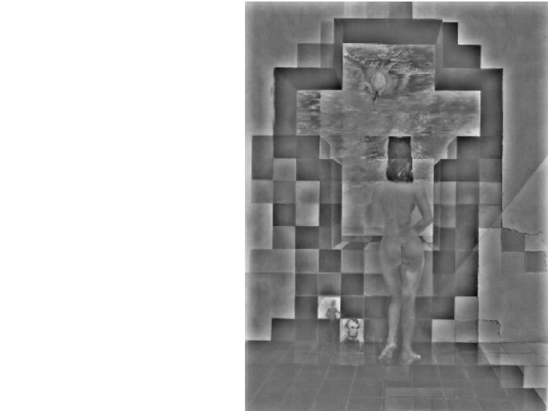
Слайд 2
Salvador Dali, “Gala Contemplating the Mediterranean Sea, which at 30 meters
becomes the portrait of Abraham Lincoln”, 1976
Salvador Dali, “Gala Contemplating the Mediterranean Sea, which at 30 meters becomes the portrait of Abraham Lincoln”, 1976
Salvador Dali
“Gala Contemplating the Mediterranean Sea,
which at 30 meters becomes the portrait
of Abraham Lincoln”, 1976

Слайд 5A nice set of basis
This change of basis has a special
name…
Teases away fast vs. slow changes in the image.

Слайд 6Jean Baptiste Joseph Fourier (1768-1830)
had crazy idea (1807):
Any univariate function can
be rewritten as a weighted sum of sines and cosines of different frequencies.
Don’t believe it?
Neither did Lagrange, Laplace, Poisson and other big wigs
Not translated into English until 1878!
But it’s (mostly) true!
called Fourier Series
there are some subtle restrictions
Don’t believe it?
Neither did Lagrange, Laplace, Poisson and other big wigs
Not translated into English until 1878!
But it’s (mostly) true!
called Fourier Series
there are some subtle restrictions
...the manner in which the author arrives at these equations is not exempt of difficulties and...his analysis to integrate them still leaves something to be desired on the score of generality and even rigour.
Laplace
Lagrange
Legendre
had crazy idea (1807): Any univariate function can be rewritten as a")
Слайд 7A sum of sines
Our building block:
Add enough of them to get
any signal f(x) you want!
How many degrees of freedom?
What does each control?
Which one encodes the coarse vs. fine structure of the signal?
How many degrees of freedom?
What does each control?
Which one encodes the coarse vs. fine structure of the signal?
 you")
Слайд 8Fourier Transform
We want to understand the frequency ω of our signal.
So, let’s reparametrize the signal by ω instead of x:
For every ω from 0 to inf, F(ω) holds the amplitude A and phase φ of the corresponding sine
How can F hold both? Complex number trick!
We can always go back:

 = sin(2pf t) + (1/3)sin(2p(3f) t)")
 = sin(2pf t) + (1/3)sin(2p(3f) t)= +")
 = sin(2pf t) + (1/3)sin(2p(3f) t)= +")


 = F(ω)")
 = f(x)")

Слайд 23Finally: Scary Math
…not really scary:
is hiding our old friend:
So it’s just
our signal f(x) times sine at frequency ω
phase can be encoded
by sin/cos pair
 times")
))));")
Слайд 25Fourier analysis in images
Intensity Image
Fourier Image
http://sharp.bu.edu/~slehar/fourier/fourier.html#filtering

Слайд 26Signals can be composed
+
=
http://sharp.bu.edu/~slehar/fourier/fourier.html#filtering
More: http://www.cs.unm.edu/~brayer/vision/fourier.html


Слайд 30The Convolution Theorem
The greatest thing since sliced (banana) bread!
The Fourier transform
of the convolution of two functions is the product of their Fourier transforms
The inverse Fourier transform of the product of two Fourier transforms is the convolution of the two inverse Fourier transforms
Convolution in spatial domain is equivalent to multiplication in frequency domain!
The inverse Fourier transform of the product of two Fourier transforms is the convolution of the two inverse Fourier transforms
Convolution in spatial domain is equivalent to multiplication in frequency domain!
 bread!The Fourier transform of the convolution of")
h(x,y)g(x,y)|F(sx,sy)||H(sx,sy)||G(sx,sy)|")
Слайд 32Why does the Gaussian give a nice smooth image, but the
square filter give edgy artifacts?
Gaussian
Box filter
Filtering


")

Слайд 41Band-pass filtering
Laplacian Pyramid (subband images)
Created from Gaussian pyramid by subtraction
Gaussian Pyramid
(low-pass images)
Created from Gaussian pyramid by subtractionGaussian Pyramid (low-pass images)")
Слайд 42Laplacian Pyramid
How can we reconstruct (collapse) this pyramid into the original
image?
Need this!
Original
image
 this pyramid into the original image?Need this!Originalimage")

Слайд 44Project 2: Hybrid Images
http://www.cs.illinois.edu/class/fa10/cs498dwh/projects/hybrid/ComputationalPhotography_ProjectHybrid.html
Gaussian Filter!
Laplacian Filter!
Project Instructions:
A. Oliva, A. Torralba,
P.G. Schyns,
“Hybrid Images,” SIGGRAPH 2006

Слайд 45Early processing in humans filters for various orientations and scales of
frequency
Perceptual cues in the mid frequencies dominate perception
When we see an image from far away, we are effectively subsampling it
Perceptual cues in the mid frequencies dominate perception
When we see an image from far away, we are effectively subsampling it
Early Visual Processing: Multi-scale edge and blob filters
Clues from Human Perception


Block-based Discrete Cosine Transform (DCT)")
Слайд 52Using DCT in JPEG
The first coefficient B(0,0) is the
DC component, the average intensity
The top-left coeffs represent low frequencies, the bottom right – high frequencies
The top-left coeffs represent low frequencies, the bottom right – high frequencies
 is the DC component, the average intensityThe")
Слайд 53Image compression using DCT
Quantize
More coarsely for high frequencies (which also
tend to have smaller values)
Many quantized high frequency values will be zero
Encode
Can decode with inverse dct
Many quantized high frequency values will be zero
Encode
Can decode with inverse dct
Quantization table
Filter responses
Quantized values

Слайд 54JPEG Compression Summary
Subsample color by factor of 2
People have bad resolution
for color
Split into blocks (8x8, typically), subtract 128
For each block
Compute DCT coefficients for
Coarsely quantize
Many high frequency components will become zero
Encode (e.g., with Huffman coding)
Split into blocks (8x8, typically), subtract 128
For each block
Compute DCT coefficients for
Coarsely quantize
Many high frequency components will become zero
Encode (e.g., with Huffman coding)
http://en.wikipedia.org/wiki/YCbCr
http://en.wikipedia.org/wiki/JPEG

Слайд 55Block size in JPEG
Block size
small block
faster
correlation exists between
neighboring pixels
large block
better compression in smooth regions
It’s 8x8 in standard JPEG
large block
better compression in smooth regions
It’s 8x8 in standard JPEG


Слайд 57Image gradient
The gradient of an image:
The gradient points in the
direction of most rapid change in intensity

Слайд 58Effects of noise
Consider a single row or column of the image
Plotting
intensity as a function of position gives a signal
Where is the edge?
How to compute a derivative?


Слайд 61Laplacian of Gaussian
Consider
Laplacian of Gaussian
operator
Where is the edge?
Zero-crossings of
bottom graph


Слайд 63Try this in MATLAB
g = fspecial('gaussian',15,2);
imagesc(g); colormap(gray);
surfl(g)
gclown = conv2(clown,g,'same');
imagesc(conv2(clown,[-1 1],'same'));
imagesc(conv2(gclown,[-1 1],'same'));
dx
= conv2(g,[-1 1],'same');
imagesc(conv2(clown,dx,'same'));
lg = fspecial('log',15,2);
lclown = conv2(clown,lg,'same');
imagesc(lclown)
imagesc(clown + .2*lclown)
imagesc(conv2(clown,dx,'same'));
lg = fspecial('log',15,2);
lclown = conv2(clown,lg,'same');
imagesc(lclown)
imagesc(clown + .2*lclown)
;imagesc(g); colormap(gray);surfl(g)gclown = conv2(clown,g,'same');imagesc(conv2(clown,[-1 1],'same'));imagesc(conv2(gclown,[-1 1],'same'));dx = conv2(g,[-1 1],'same');imagesc(conv2(clown,dx,'same'));lg =")