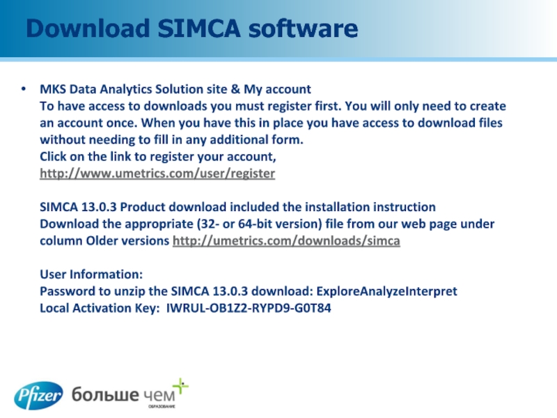
have access to downloads you must register first. You will only need to create an account once. When you have this in place you have access to download files without needing to fill in any additional form.
Click on the link to register your account, http://www.umetrics.com/user/register
SIMCA 13.0.3 Product download included the installation instruction
Download the appropriate (32- or 64-bit version) file from our web page under column Older versions http://umetrics.com/downloads/simca
User Information:
Password to unzip the SIMCA 13.0.3 download: ExploreAnalyzeInterpret
Local Activation Key: IWRUL-OB1Z2-RYPD9-G0T84
- Главная
- Разное
- Дизайн
- Бизнес и предпринимательство
- Аналитика
- Образование
- Развлечения
- Красота и здоровье
- Финансы
- Государство
- Путешествия
- Спорт
- Недвижимость
- Армия
- Графика
- Культурология
- Еда и кулинария
- Лингвистика
- Английский язык
- Астрономия
- Алгебра
- Биология
- География
- Детские презентации
- Информатика
- История
- Литература
- Маркетинг
- Математика
- Медицина
- Менеджмент
- Музыка
- МХК
- Немецкий язык
- ОБЖ
- Обществознание
- Окружающий мир
- Педагогика
- Русский язык
- Технология
- Физика
- Философия
- Химия
- Шаблоны, картинки для презентаций
- Экология
- Экономика
- Юриспруденция
Download SIMCA software презентация
Содержание
- 1. Download SIMCA software
- 2. Background information Drying process after wet granulation
- 3. What we will do Try to find
- 4. Multivariable Regression Multivariable regression enables you to
- 5. Step 1 Launch Microsoft Excel and click
- 6. Step 2 Click the "Add-Ins" item in
- 7. Step 3 Tick the check box
- 8. Step 4 & 5 Enter your column
- 9. Step 6 Scroll through the list
- 10. Step 7 Type the location of
- 11. Step 8 Enter the location of
- 12. Step 9 & 10 Click on
- 13. Step 11 Choose options from the
- 14. Step 12 Click on the "OK" button
- 15. Coefficients The next stage is the coefficients.
- 16. Different Plots The Residual Plot graphs
- 17. Inserting a Scatter Diagram into Excel
- 18. Add a Trendline to Excel You
- 19. Formatting an Excel Trendline To format
- 20. Simple Linear Regression Using an Excel
- 21. Simple Linear Regression In array one, fill
- 22. Linear Regression Formula Repeat the same process
- 23. Linear Regression Formula The intercept point is
- 24. Chart
Слайд 2Background information
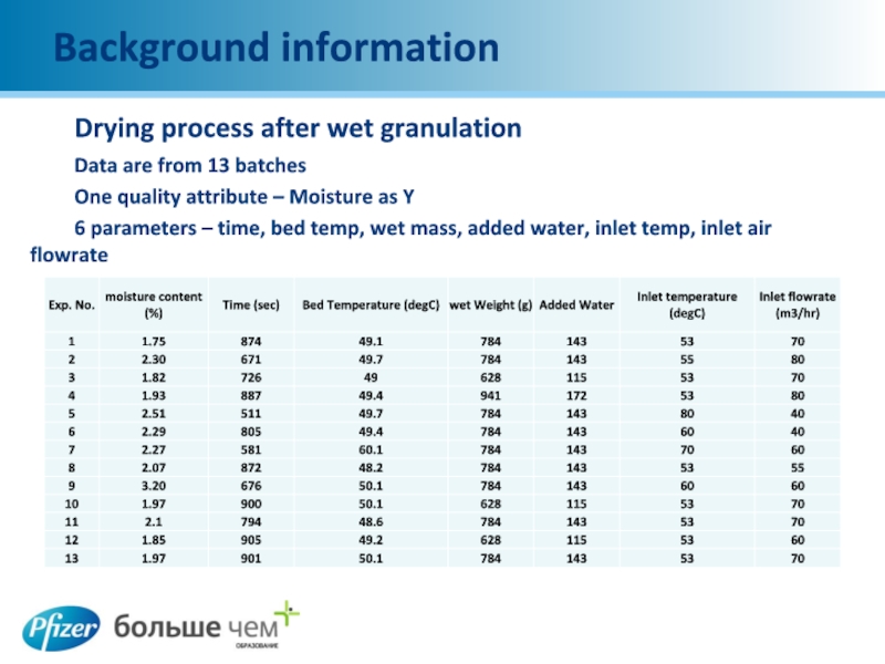
Drying process after wet granulation
Data are from 13 batches
One quality
attribute – Moisture as Y
6 parameters – time, bed temp, wet mass, added water, inlet temp, inlet air flowrate
6 parameters – time, bed temp, wet mass, added water, inlet temp, inlet air flowrate
Слайд 3What we will do
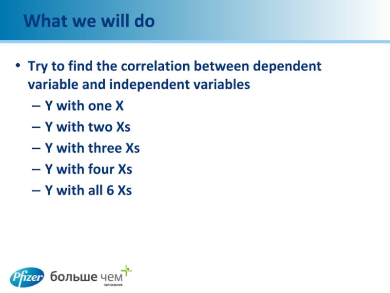
Try to find the correlation between dependent variable
and independent variables
Y with one X
Y with two Xs
Y with three Xs
Y with four Xs
Y with all 6 Xs
Y with one X
Y with two Xs
Y with three Xs
Y with four Xs
Y with all 6 Xs
Слайд 4Multivariable Regression
Multivariable regression enables you to relate one dependent variable to
multiple independent variables you've derived from measurements. This type of data analysis helps you search for the effects of your observed data on a related condition or predict a condition based on other related observations.
Слайд 5Step 1
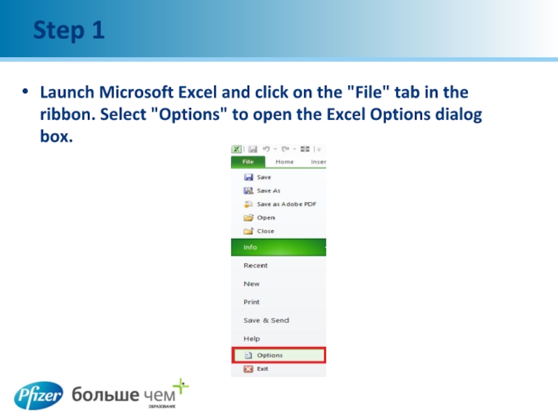
Launch Microsoft Excel and click on the "File" tab in
the ribbon. Select "Options" to open the Excel Options dialog box.
Слайд 6Step 2
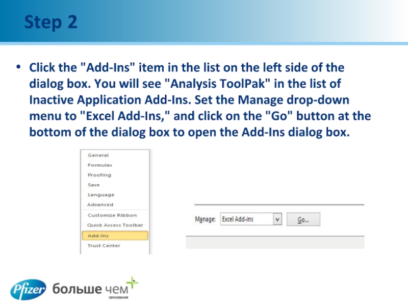
Click the "Add-Ins" item in the list on the left
side of the dialog box. You will see "Analysis ToolPak" in the list of Inactive Application Add-Ins. Set the Manage drop-down menu to "Excel Add-Ins," and click on the "Go" button at the bottom of the dialog box to open the Add-Ins dialog box.
Слайд 7Step 3
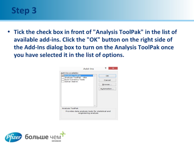
Tick the check box in front of "Analysis ToolPak" in
the list of available add-ins. Click the "OK" button on the right side of the Add-Ins dialog box to turn on the Analysis ToolPak once you have selected it in the list of options.
Слайд 8Step 4 & 5
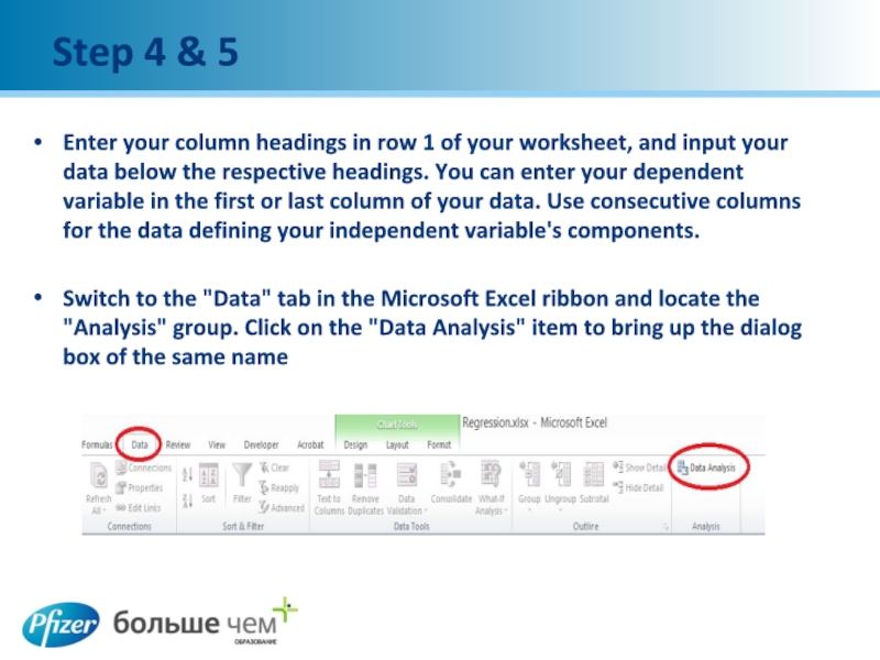
Enter your column headings in row 1 of
your worksheet, and input your data below the respective headings. You can enter your dependent variable in the first or last column of your data. Use consecutive columns for the data defining your independent variable's components.
Switch to the "Data" tab in the Microsoft Excel ribbon and locate the "Analysis" group. Click on the "Data Analysis" item to bring up the dialog box of the same name
Switch to the "Data" tab in the Microsoft Excel ribbon and locate the "Analysis" group. Click on the "Data Analysis" item to bring up the dialog box of the same name
Слайд 9Step 6
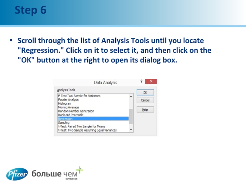
Scroll through the list of Analysis Tools until you locate
"Regression." Click on it to select it, and then click on the "OK" button at the right to open its dialog box.
Слайд 10Step 7
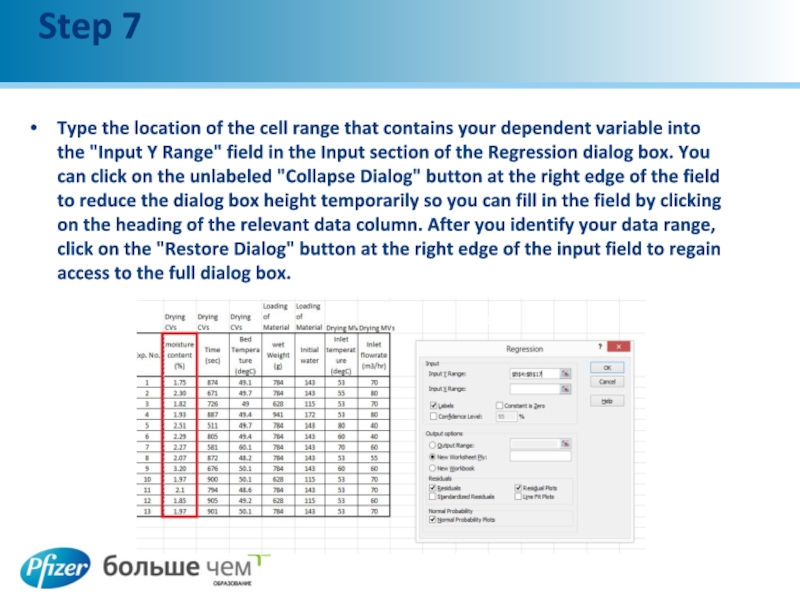
Type the location of the cell range that contains your
dependent variable into the "Input Y Range" field in the Input section of the Regression dialog box. You can click on the unlabeled "Collapse Dialog" button at the right edge of the field to reduce the dialog box height temporarily so you can fill in the field by clicking on the heading of the relevant data column. After you identify your data range, click on the "Restore Dialog" button at the right edge of the input field to regain access to the full dialog box.
Слайд 11Step 8
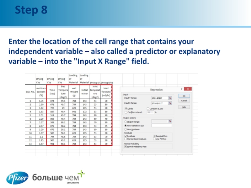
Enter the location of the cell range that contains your
independent variable – also called a predictor or explanatory variable – into the "Input X Range" field.
Слайд 12Step 9 & 10
Click on the "Labels" check box to tell
Excel that the first row of your data contains data labels. If you didn't enter a header row, leave this box unchecked.
Click on the "Output Range" radio button in the Output Options section of the dialog box and enter a data range in the entry field to identify a location in your current worksheet for the output of your analysis. Use the "Collapse Dialog" and "Restore Dialog" buttons to click through your worksheet and identify where to put your results. Select the "New Worksheet Ply" radio button to place your results in a new sheet within your workbook, or choose "New Workbook" to put the results in a new file.
Click on the "Output Range" radio button in the Output Options section of the dialog box and enter a data range in the entry field to identify a location in your current worksheet for the output of your analysis. Use the "Collapse Dialog" and "Restore Dialog" buttons to click through your worksheet and identify where to put your results. Select the "New Worksheet Ply" radio button to place your results in a new sheet within your workbook, or choose "New Workbook" to put the results in a new file.
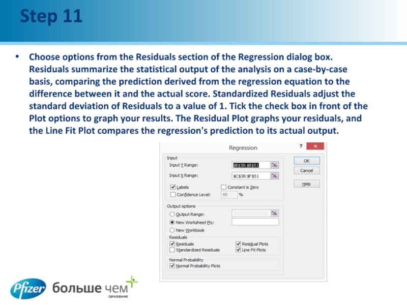
Слайд 13Step 11
Choose options from the Residuals section of the Regression dialog
box. Residuals summarize the statistical output of the analysis on a case-by-case basis, comparing the prediction derived from the regression equation to the difference between it and the actual score. Standardized Residuals adjust the standard deviation of Residuals to a value of 1. Tick the check box in front of the Plot options to graph your results. The Residual Plot graphs your residuals, and the Line Fit Plot compares the regression's prediction to its actual output.
Слайд 14Step 12
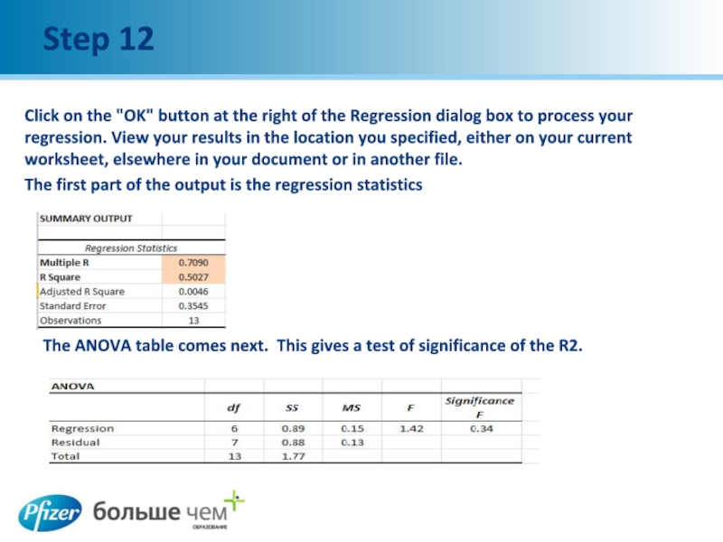
Click on the "OK" button at the right of the
Regression dialog box to process your regression. View your results in the location you specified, either on your current worksheet, elsewhere in your document or in another file.
The first part of the output is the regression statistics
The first part of the output is the regression statistics
The ANOVA table comes next. This gives a test of significance of the R2.
Слайд 15Coefficients
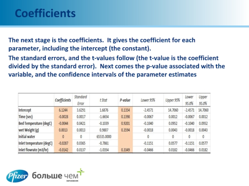
The next stage is the coefficients. It gives the coefficient for
each parameter, including the intercept (the constant).
The standard errors, and the t-values follow (the t-value is the coefficient divided by the standard error). Next comes the p-value associated with the variable, and the confidence intervals of the parameter estimates
The standard errors, and the t-values follow (the t-value is the coefficient divided by the standard error). Next comes the p-value associated with the variable, and the confidence intervals of the parameter estimates
Слайд 16Different Plots
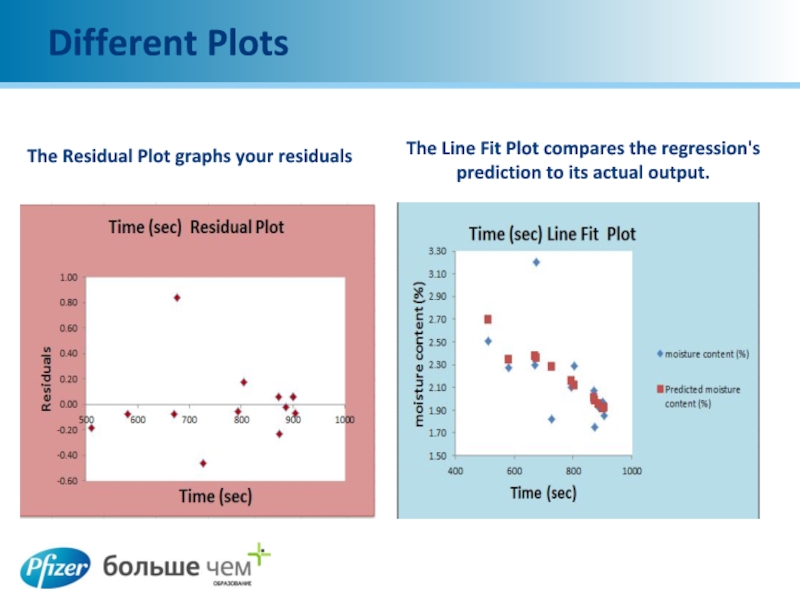
The Residual Plot graphs your residuals
The Line Fit Plot compares
the regression's prediction to its actual output.
Слайд 17Inserting a Scatter Diagram into Excel
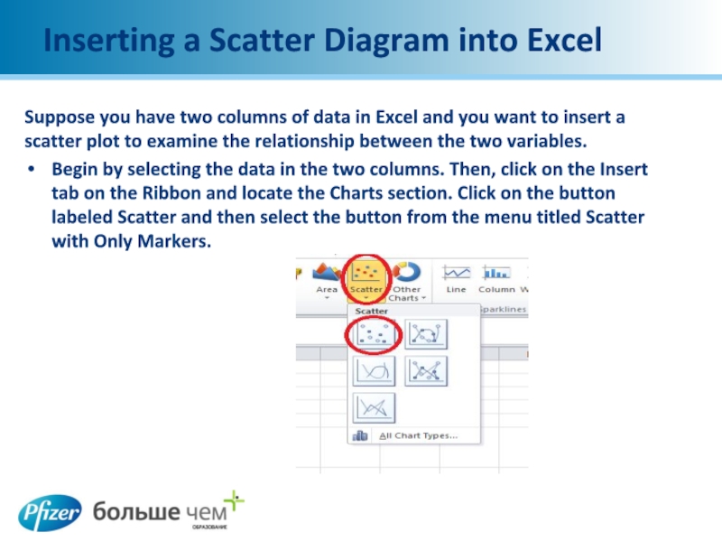
Suppose you have two columns of
data in Excel and you want to insert a scatter plot to examine the relationship between the two variables.
Begin by selecting the data in the two columns. Then, click on the Insert tab on the Ribbon and locate the Charts section. Click on the button labeled Scatter and then select the button from the menu titled Scatter with Only Markers.
Begin by selecting the data in the two columns. Then, click on the Insert tab on the Ribbon and locate the Charts section. Click on the button labeled Scatter and then select the button from the menu titled Scatter with Only Markers.
Слайд 18Add a Trendline to Excel
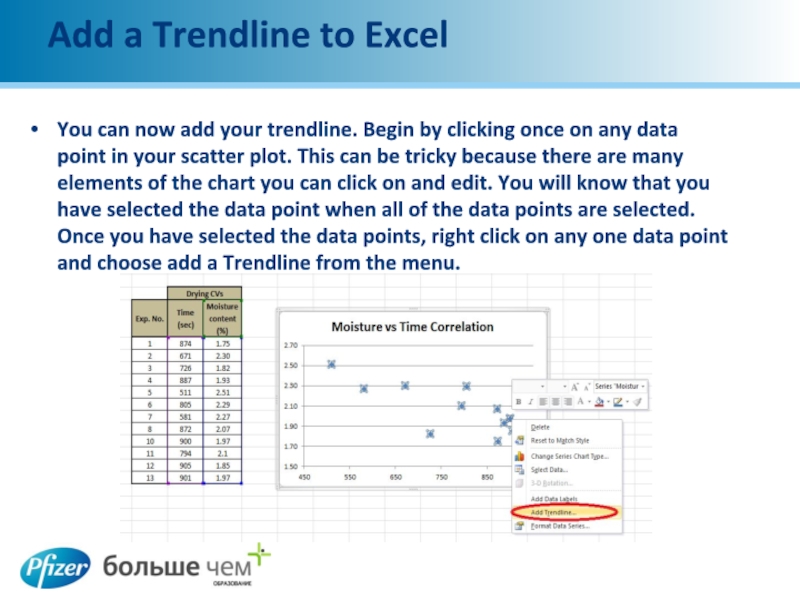
You can now add your trendline. Begin
by clicking once on any data point in your scatter plot. This can be tricky because there are many elements of the chart you can click on and edit. You will know that you have selected the data point when all of the data points are selected. Once you have selected the data points, right click on any one data point and choose add a Trendline from the menu.
Слайд 19Formatting an Excel Trendline
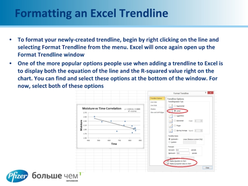
To format your newly-created trendline, begin by right
clicking on the line and selecting Format Trendline from the menu. Excel will once again open up the Format Trendline window
One of the more popular options people use when adding a trendline to Excel is to display both the equation of the line and the R-squared value right on the chart. You can find and select these options at the bottom of the window. For now, select both of these options
One of the more popular options people use when adding a trendline to Excel is to display both the equation of the line and the R-squared value right on the chart. You can find and select these options at the bottom of the window. For now, select both of these options
Слайд 20Simple Linear Regression
Using an Excel function
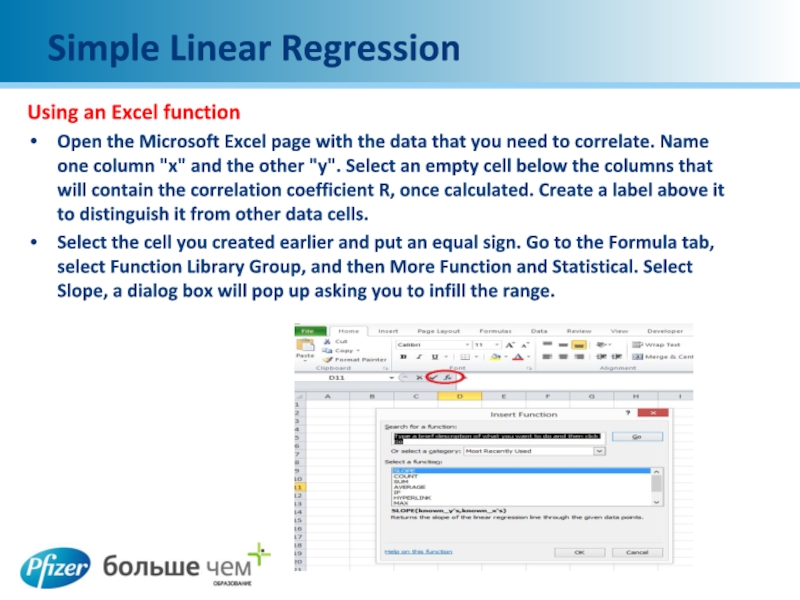
Open the Microsoft Excel page with
the data that you need to correlate. Name one column "x" and the other "y". Select an empty cell below the columns that will contain the correlation coefficient R, once calculated. Create a label above it to distinguish it from other data cells.
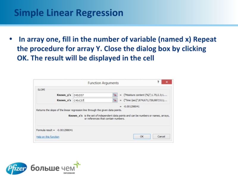
Select the cell you created earlier and put an equal sign. Go to the Formula tab, select Function Library Group, and then More Function and Statistical. Select Slope, a dialog box will pop up asking you to infill the range.
Select the cell you created earlier and put an equal sign. Go to the Formula tab, select Function Library Group, and then More Function and Statistical. Select Slope, a dialog box will pop up asking you to infill the range.
Слайд 21Simple Linear Regression
In array one, fill in the number of variable
(named x) Repeat the procedure for array Y. Close the dialog box by clicking OK. The result will be displayed in the cell
Слайд 22Linear Regression Formula
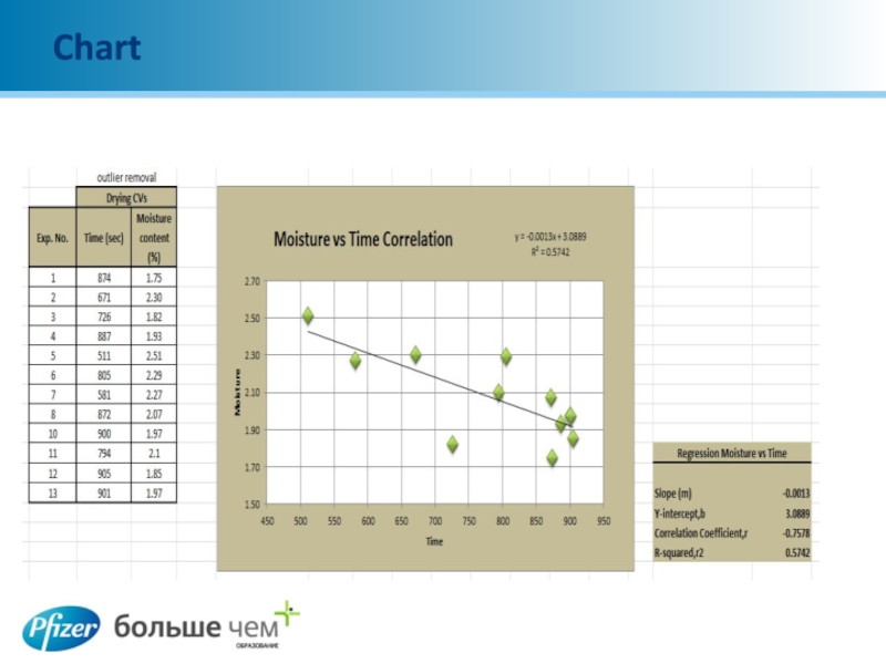
Repeat the same process to get result for Intercept
- Correlation and R- Squared
The syntax to calculate each of the terms in the regression is as follows:
The SLOPE function returns the slope of the linear regression line that is used to predict Y values from X values.
Slope,m: =SLOPE(Known_Y’s,Known_x’s)
The syntax to calculate each of the terms in the regression is as follows:
The SLOPE function returns the slope of the linear regression line that is used to predict Y values from X values.
Slope,m: =SLOPE(Known_Y’s,Known_x’s)
Слайд 23Linear Regression Formula
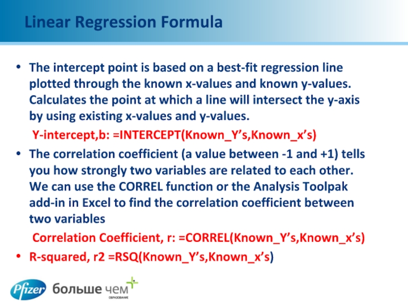
The intercept point is based on a best-fit regression
line plotted through the known x-values and known y-values. Calculates the point at which a line will intersect the y-axis by using existing x-values and y-values.
Y-intercept,b: =INTERCEPT(Known_Y’s,Known_x’s)
The correlation coefficient (a value between -1 and +1) tells you how strongly two variables are related to each other. We can use the CORREL function or the Analysis Toolpak add-in in Excel to find the correlation coefficient between two variables
Correlation Coefficient, r: =CORREL(Known_Y’s,Known_x’s)
R-squared, r2 =RSQ(Known_Y’s,Known_x’s)
