- Главная
- Разное
- Дизайн
- Бизнес и предпринимательство
- Аналитика
- Образование
- Развлечения
- Красота и здоровье
- Финансы
- Государство
- Путешествия
- Спорт
- Недвижимость
- Армия
- Графика
- Культурология
- Еда и кулинария
- Лингвистика
- Английский язык
- Астрономия
- Алгебра
- Биология
- География
- Детские презентации
- Информатика
- История
- Литература
- Маркетинг
- Математика
- Медицина
- Менеджмент
- Музыка
- МХК
- Немецкий язык
- ОБЖ
- Обществознание
- Окружающий мир
- Педагогика
- Русский язык
- Технология
- Физика
- Философия
- Химия
- Шаблоны, картинки для презентаций
- Экология
- Экономика
- Юриспруденция
Cmpe 466 computer graphics. 2d geometric transformations. (Chapter 7) презентация
Содержание
- 1. Cmpe 466 computer graphics. 2d geometric transformations. (Chapter 7)
- 2. Basic geometric transformations Translation Rotation Scaling
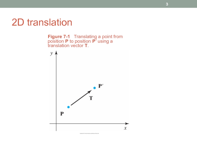
- 3. 2D translation Figure 7-1 Translating a
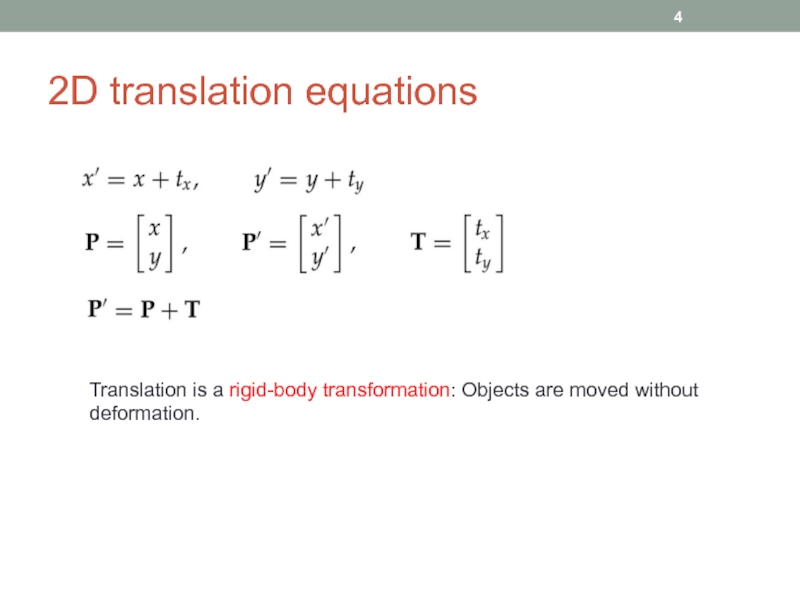
- 4. 2D translation equations Translation is a rigid-body transformation: Objects are moved without deformation.
- 5. 2D translation example Figure 7-2 Moving
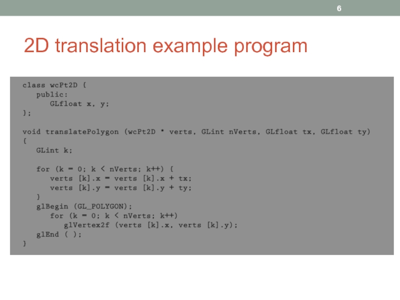
- 6. 2D translation example program
- 7. 2D rotation All points of the object
- 8. 2D rotation Figure 7-4 Rotation of
- 9. 2D rotation in matrix form Rotation is
- 10. Rotation about a general pivot point Figure
- 11. 2D rotation example // Make necessary allocations!!
- 12. 2D scaling sx and sy are scaling
- 13. 2D scaling Figure 7-6 Turning a
- 14. 2D scaling Figure 7-7 A line
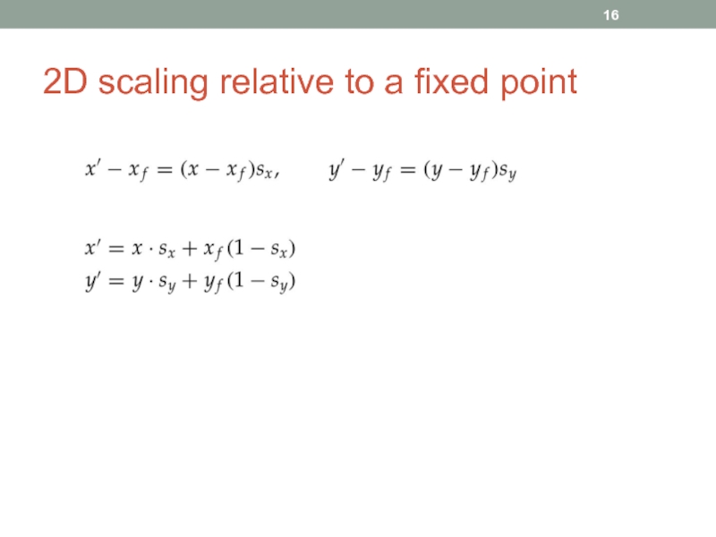
- 15. Scaling relative to a fixed point Figure
- 16. 2D scaling relative to a fixed point
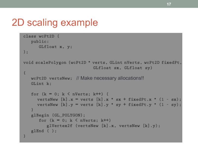
- 17. 2D scaling example // Make necessary allocations!!
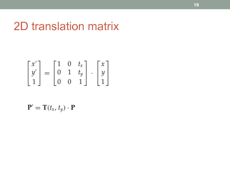
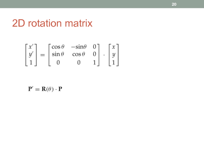
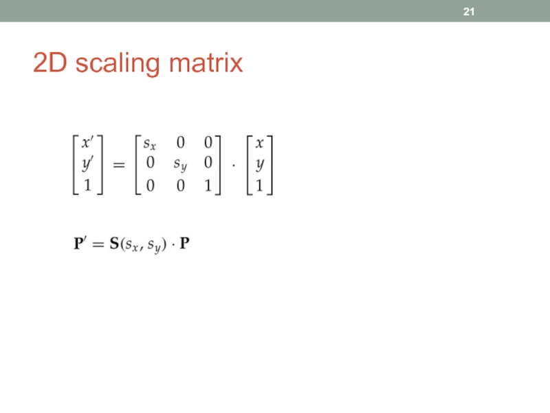
- 18. Matrix representations and homogeneous coordinates Multiplicative and
- 19. 2D translation matrix
- 20. 2D rotation matrix
- 21. 2D scaling matrix
- 22. Inverse transformations Inverse translation Inverse rotation Inverse scaling
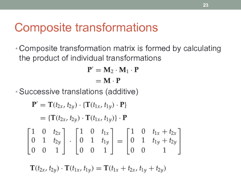
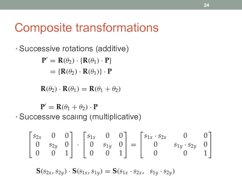
- 23. Composite transformations Composite transformation matrix is formed
- 24. Composite transformations Successive rotations (additive) Successive scaling (multiplicative)
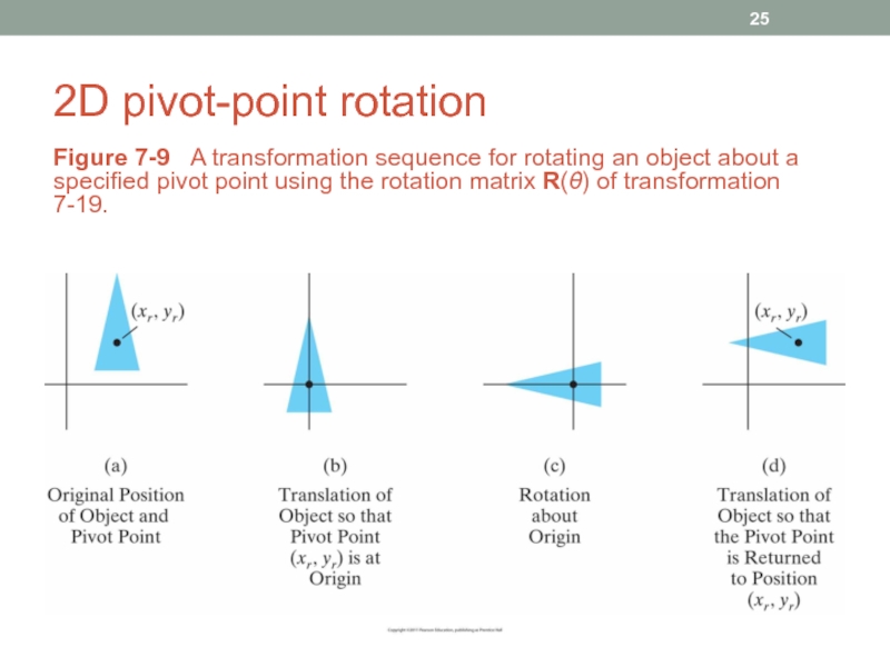
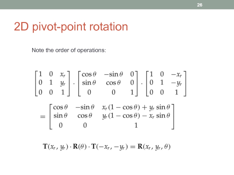
- 25. 2D pivot-point rotation Figure 7-9 A
- 26. 2D pivot-point rotation Note the order of operations:
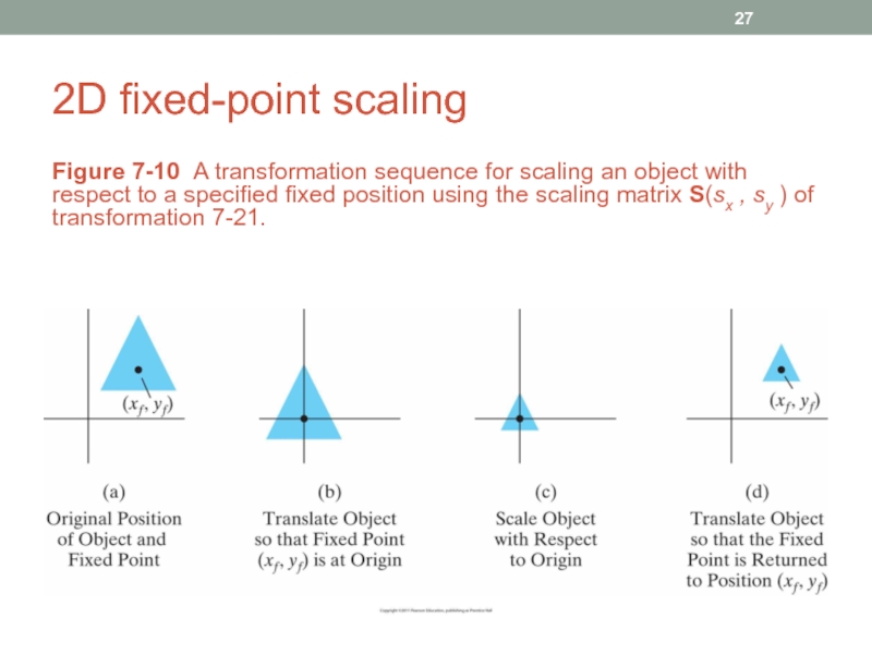
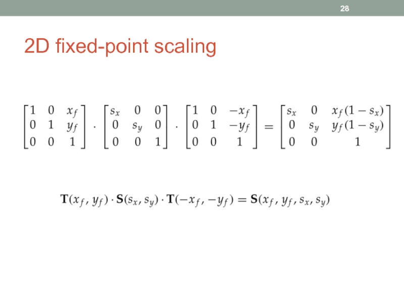
- 27. 2D fixed-point scaling Figure 7-10 A transformation
- 28. 2D fixed-point scaling
- 29. Matrix concatenation properties Multiplication is associative
- 30. Computational efficiency Formulation of a concatenated matrix
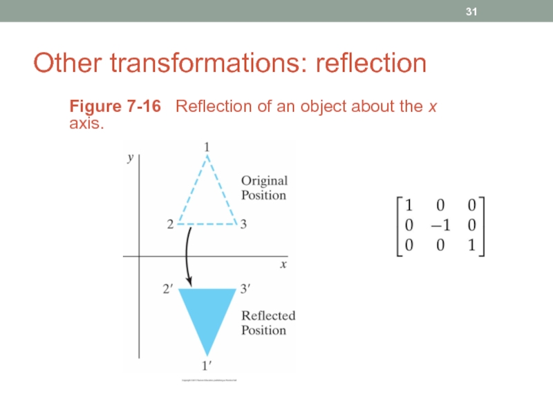
- 31. Other transformations: reflection Figure 7-16 Reflection of an object about the x axis.
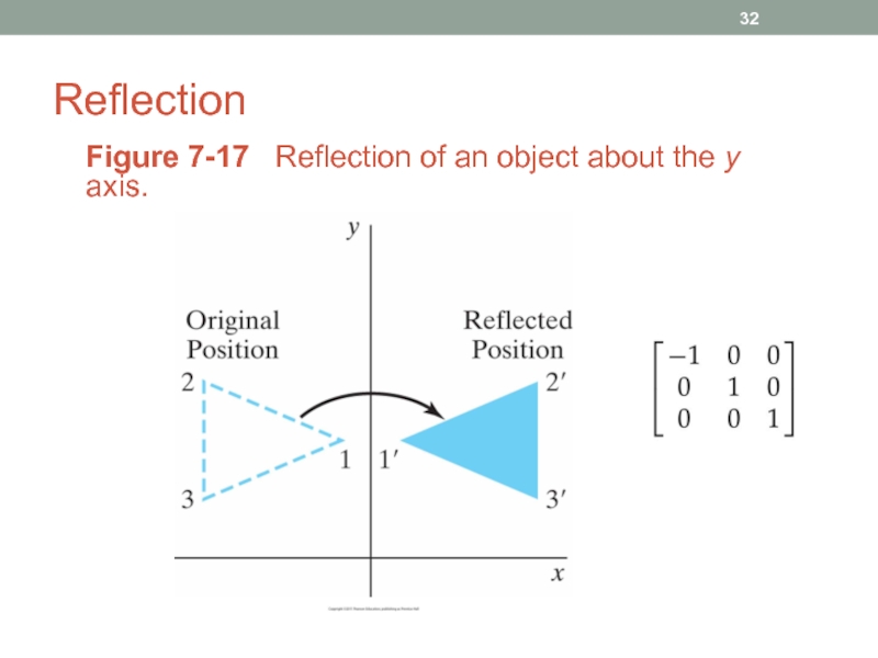
- 32. Reflection Figure 7-17 Reflection of an object about the y axis.
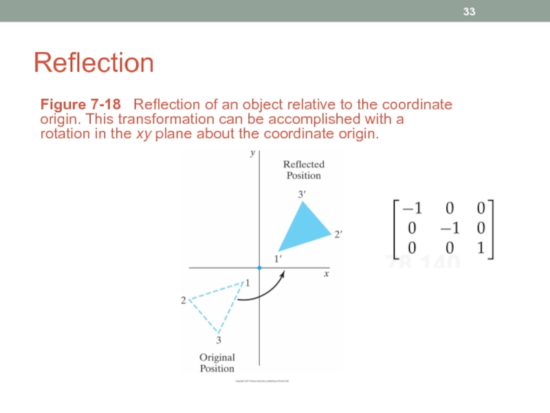
- 33. Reflection Figure 7-18 Reflection of an
- 34. Reflection Figure 7-19 Reflection of an
- 35. Reflection Figure 7-20 Reflection of an
- 36. Other transformations: shear Distorts the shape of
- 37. Shear Figure 7-24 A unit square
- 38. Shear Figure 7-25 A unit square
- 39. Transformations between 2D coordinate systems Figure 7-30
- 40. Transformations x’y’ system can be obtained by
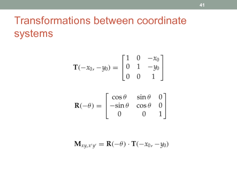
- 41. Transformations between coordinate systems
- 42. Alternative method Figure 7-32 Cartesian system
- 43. Transformations Figure 7-33 A Cartesian x
- 44. Example: Rotating points vs. rotating coordinate systems
- 45. Example continued You may think of this
- 46. Example continued Now consider the point P=(x(2),y(2),1)T
- 47. OpenGL matrix operations glMatrixMode ( GL_MODELVIEW )
- 48. OpenGL transformation example
- 49. OpenGL transformation example Figure 7-34 Translating
- 50. OpenGL transformation example Figure 7-35 Rotating
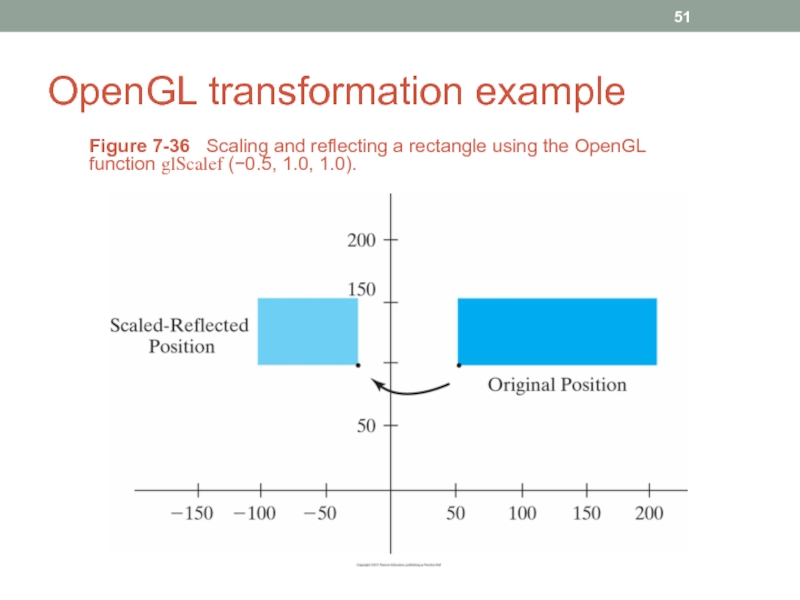
- 51. OpenGL transformation example Figure 7-36 Scaling
Слайд 1CMPE 466
COMPUTER GRAPHICS
Chapter 7
2D Geometric Transformations
Instructor: D. Arifler
Material based on
- Computer
Fundamentals of Computer Graphics, Third Edition by by Peter Shirley and Steve Marschner
Computer Graphics by F. S. Hill
Слайд 32D translation
Figure 7-1 Translating a point from position P to
Слайд 42D translation equations
Translation is a rigid-body transformation: Objects are moved without
deformation.
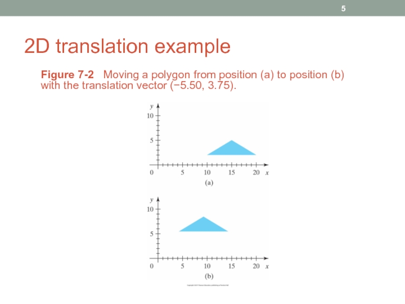
Слайд 52D translation example
Figure 7-2 Moving a polygon from position (a)
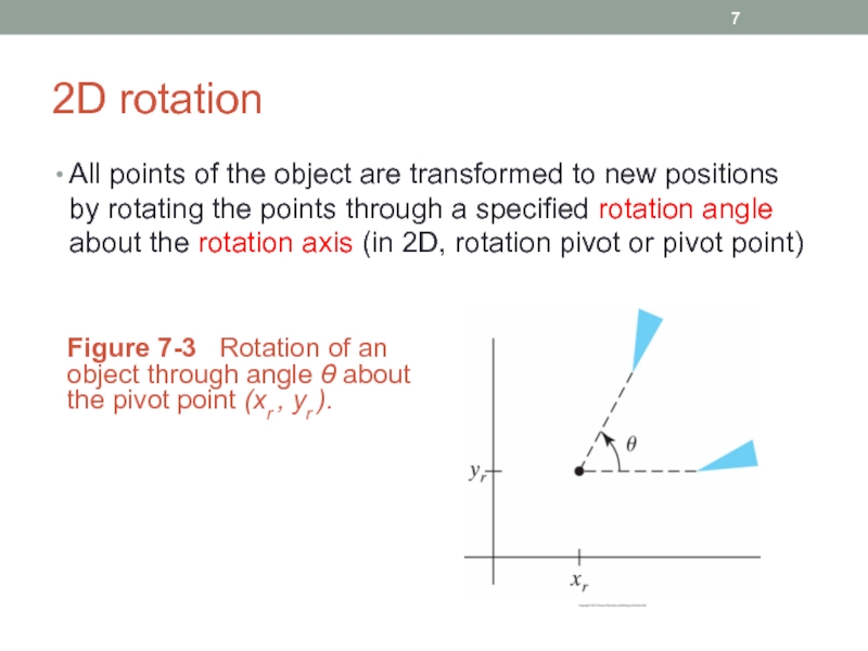
Слайд 72D rotation
All points of the object are transformed to new positions
Figure 7-3 Rotation of an object through angle θ about the pivot point (xr , yr ).
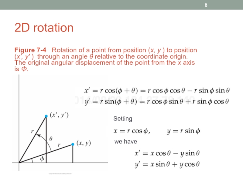
Слайд 82D rotation
Figure 7-4 Rotation of a point from position (x,
Setting
we have
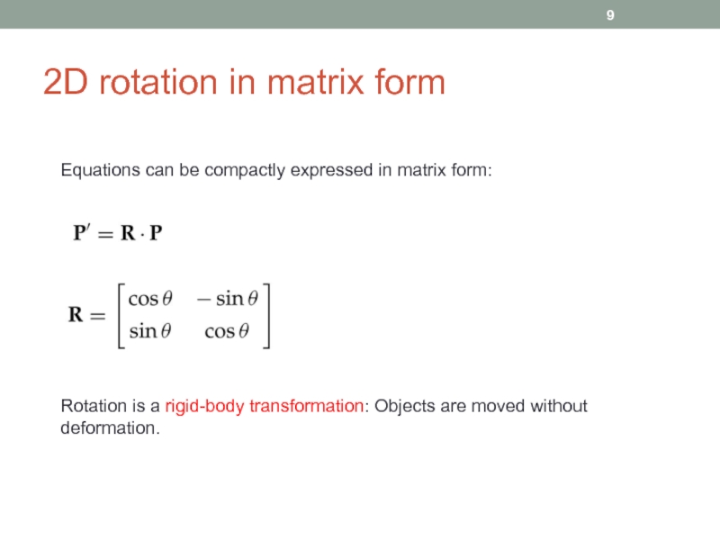
Слайд 92D rotation in matrix form
Rotation is a rigid-body transformation: Objects are
deformation.
Equations can be compactly expressed in matrix form:
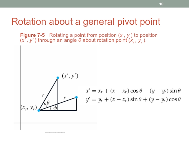
Слайд 10Rotation about a general pivot point
Figure 7-5 Rotating a point
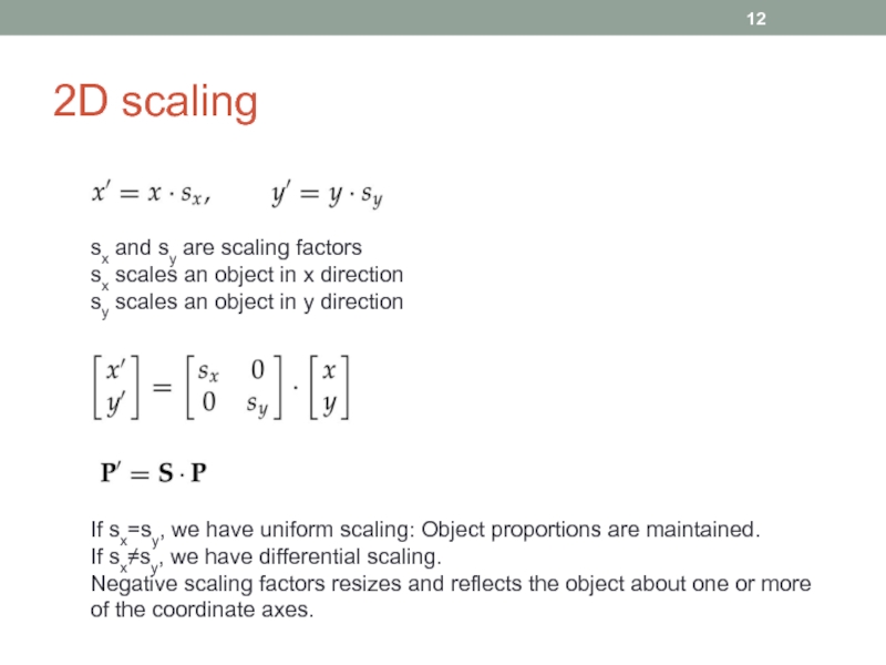
Слайд 122D scaling
sx and sy are scaling factors
sx scales an object in
sy scales an object in y direction
If sx=sy, we have uniform scaling: Object proportions are maintained.
If sx≠sy, we have differential scaling.
Negative scaling factors resizes and reflects the object about one or more
of the coordinate axes.
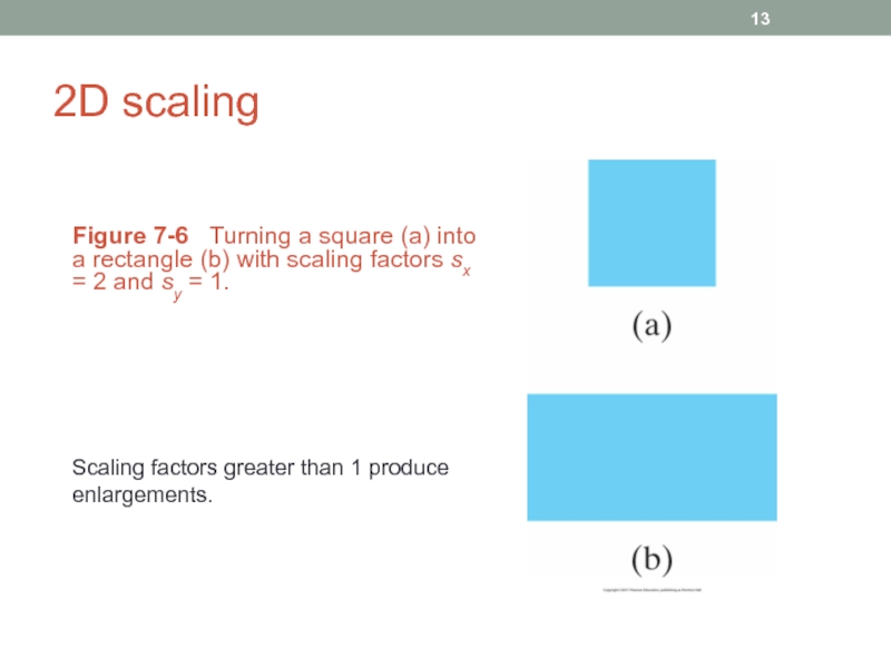
Слайд 132D scaling
Figure 7-6 Turning a square (a) into a rectangle
Scaling factors greater than 1 produce
enlargements.
Слайд 142D scaling
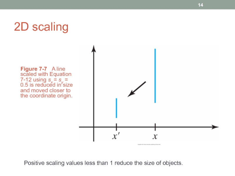
Figure 7-7 A line scaled with Equation 7-12 using
Positive scaling values less than 1 reduce the size of objects.
Слайд 15Scaling relative to a fixed point
Figure 7-8 Scaling relative to
Fixed point remains
unchanged after the
scaling transformation.
Слайд 18Matrix representations and homogeneous coordinates
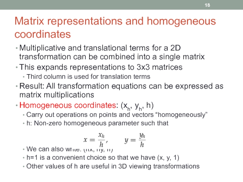
Multiplicative and translational terms for a 2D
This expands representations to 3x3 matrices
Third column is used for translation terms
Result: All transformation equations can be expressed as matrix multiplications
Homogeneous coordinates: (xh, yh, h)
Carry out operations on points and vectors “homogeneously”
h: Non-zero homogeneous parameter such that
We can also write: (hx, hy, h)
h=1 is a convenient choice so that we have (x, y, 1)
Other values of h are useful in 3D viewing transformations
Слайд 23Composite transformations
Composite transformation matrix is formed by calculating the product of
Successive translations (additive)
Слайд 252D pivot-point rotation
Figure 7-9 A transformation sequence for rotating an
Слайд 272D fixed-point scaling
Figure 7-10 A transformation sequence for scaling an object
Слайд 29Matrix concatenation properties
Multiplication is associative
Multiplication is NOT commutative
Unless the sequence of
M2M1 is not equal to M1M2 in general
Слайд 30Computational efficiency
Formulation of a concatenated matrix may be more efficient
Requires fewer
Rotation calculations require trigonometric evaluations
In animations with small-angle rotations, approximations (e.g. power series) and iterative calculations can reduce complexity
Слайд 33Reflection
Figure 7-18 Reflection of an object relative to the coordinate
Слайд 34Reflection
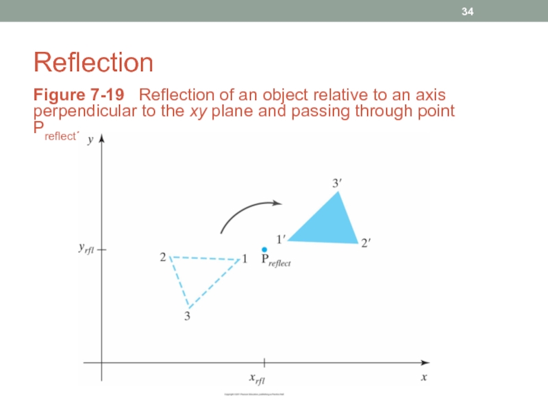
Figure 7-19 Reflection of an object relative to an axis
Слайд 36Other transformations: shear
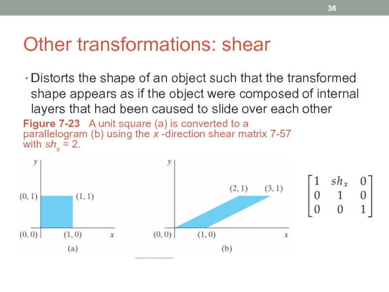
Distorts the shape of an object such that the
Figure 7-23 A unit square (a) is converted to a parallelogram (b) using the x -direction shear matrix 7-57 with shx = 2.
Слайд 37Shear
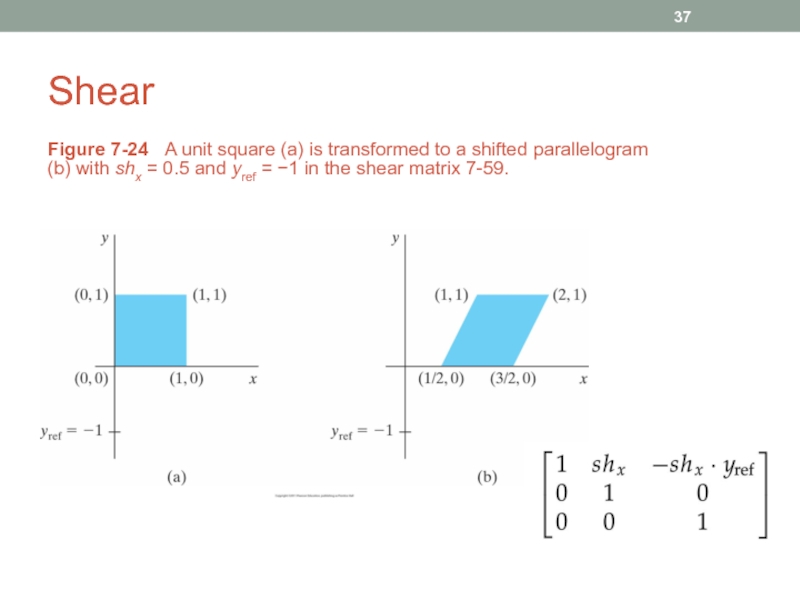
Figure 7-24 A unit square (a) is transformed to a
Слайд 38Shear
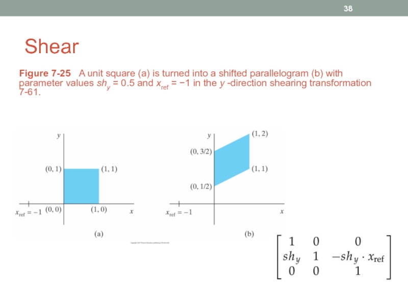
Figure 7-25 A unit square (a) is turned into a
Слайд 39Transformations between 2D coordinate systems
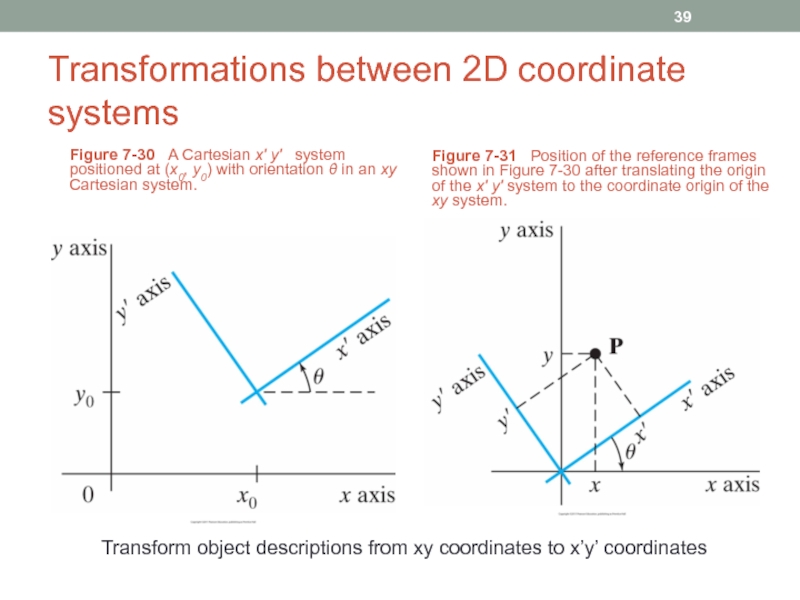
Figure 7-30 A Cartesian x' y'
Figure 7-31 Position of the reference frames shown in Figure 7-30 after translating the origin of the x' y' system to the coordinate origin of the xy system.
Transform object descriptions from xy coordinates to x’y’ coordinates
Слайд 40Transformations
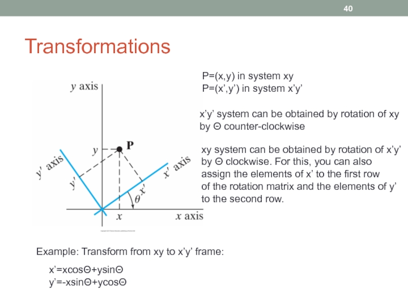
x’y’ system can be obtained by rotation of xy
by Θ counter-clockwise
xy
by Θ clockwise. For this, you can also
assign the elements of x’ to the first row
of the rotation matrix and the elements of y’
to the second row.
P=(x,y) in system xy
P=(x’,y’) in system x’y’
x’=xcosΘ+ysinΘ
y’=-xsinΘ+ycosΘ
Example: Transform from xy to x’y’ frame:
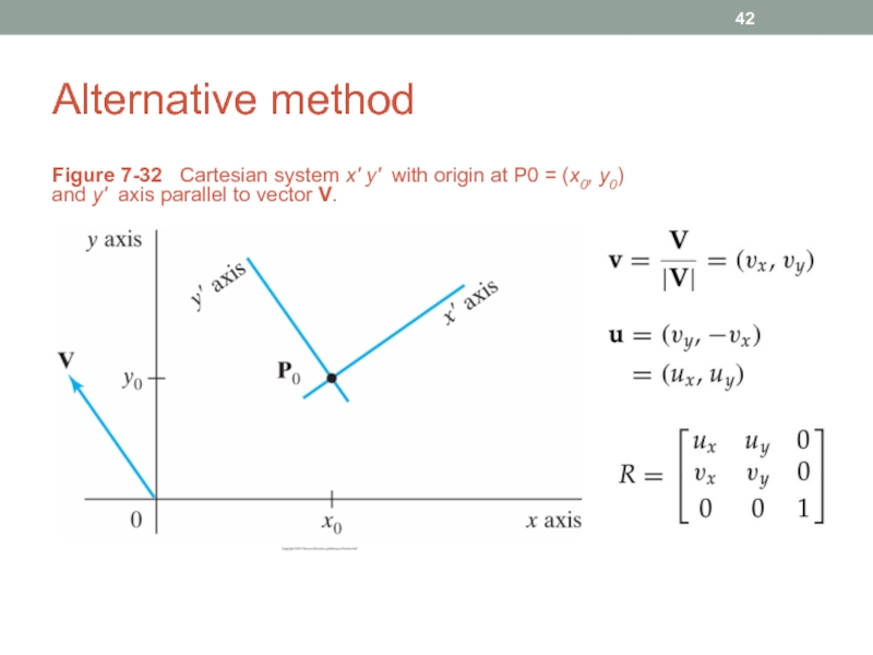
Слайд 42Alternative method
Figure 7-32 Cartesian system x' y' with origin at
Слайд 43Transformations
Figure 7-33 A Cartesian x ' y' system defined with
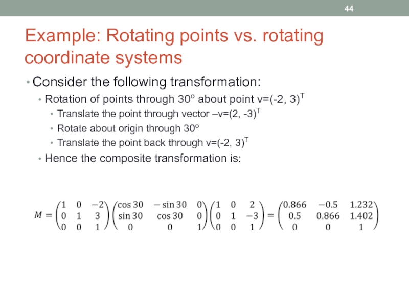
Слайд 44Example: Rotating points vs. rotating coordinate systems
Consider the following transformation:
Rotation of
Translate the point through vector –v=(2, -3)T
Rotate about origin through 30o
Translate the point back through v=(-2, 3)T
Hence the composite transformation is:
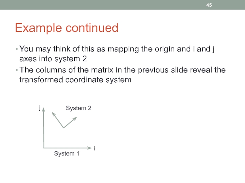
Слайд 45Example continued
You may think of this as mapping the origin and
The columns of the matrix in the previous slide reveal the transformed coordinate system
i
j
System 1
System 2
Слайд 46Example continued
Now consider the point P=(x(2),y(2),1)T in System 2
What are the
The answer is MP
For example, (1, 2, 1)T in System 2 lies at (1.098, 3.634,1)T in System 1
Now, consider the point P=(x(1),y(1),1)T in System 1
What are the coordinates of this point expressed in terms of System 2?
The answer is M-1P
Слайд 47OpenGL matrix operations
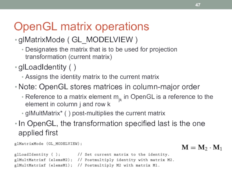
glMatrixMode ( GL_MODELVIEW )
Designates the matrix that is to
glLoadIdentity ( )
Assigns the identity matrix to the current matrix
Note: OpenGL stores matrices in column-major order
Reference to a matrix element mjk in OpenGL is a reference to the element in column j and row k
glMultMatrix* ( ) post-multiplies the current matrix
In OpenGL, the transformation specified last is the one applied first
