automatically regulate a process to maintain a desired outcome. Automatic controls are designed to handle dynamic situations where there are unplanned changes. The three components of an automatic control system are the process variable, the control variable, and the controller.
A process variable is the dependent variable that is to be controlled in a control system.
A control variable or manipulated variable, is the independent variable that is used to adjust the dependent variable,the process variable.
A controller is a device that compares a process measurement to a setpoint and changes the control variable (CV) to bring the process variable (PV) back to the setpoint.
- Главная
- Разное
- Дизайн
- Бизнес и предпринимательство
- Аналитика
- Образование
- Развлечения
- Красота и здоровье
- Финансы
- Государство
- Путешествия
- Спорт
- Недвижимость
- Армия
- Графика
- Культурология
- Еда и кулинария
- Лингвистика
- Английский язык
- Астрономия
- Алгебра
- Биология
- География
- Детские презентации
- Информатика
- История
- Литература
- Маркетинг
- Математика
- Медицина
- Менеджмент
- Музыка
- МХК
- Немецкий язык
- ОБЖ
- Обществознание
- Окружающий мир
- Педагогика
- Русский язык
- Технология
- Физика
- Философия
- Химия
- Шаблоны, картинки для презентаций
- Экология
- Экономика
- Юриспруденция
Automatic control system презентация
Содержание
- 1. Automatic control system
- 2. An automatic control system adds two elements
- 3. An automative cruise control is an example
- 4. Self regulation Some automatic processes are self
- 5. An example of process that is not self-regulating is chemical reaction.
- 7. Process dynamics The degree of difficulty
- 9. Process Gain Gain is a ratio
- 10. Lags A lag is a delay
- 12. Dead time Dead time is the
- 13. Control functions Controllers are made up of
- 16. Control actions Direct action is a form
- 21. Bumpless transfer Bumpless transfer is a controller
- 23. Controller Algorithms The actions of controllers can
- 24. A common example of a discrete controller
- 26. MULTISTEP CONTROLLERS Multistep controllers are controllers
- 27. CONTINUOUS CONTROLLERS Controllers automatically compare the
- 29. Why Controllers Need Tuning? Controllers are tuned
- 30. Examples: Change in Input to Controller -
- 31. PROPORTIONAL ACTION Proportional (P) control is method
- 33. PROPORTIONAL BAND Proportional Band (PB) is another
- 38. Proportional, Derivative Control The
- 39. INTEGRAL (I) CONTROL (RESET) Duration of Error
- 42. DERIVATIVE CONTROL Derivative Mode Basics - Some
- 43. Derivative Mode Example - Let's start a
- 45. Proportional+Integral+Derivative Control Although PD control deals
- 46. The Characteristics of P, I, and D
- 47. Proportional Control By only employing proportional control,
- 48. The Characteristics of P, I, and D controllers
- 49. Tips for Designing a PID Controller
- 50. Not every process requires a full PID
- 51. By using all three control algorithms
- 52. Cascade (Remote Setpoint controllers) Cascade control is
- 53. Ratio control Ratio control loops are designed
- 54. Feedforward control Feedforward control is a
- 55. Digital controllers A digital controller is a
- 57. Direct Computer Control System A direct computer
- 58. Distributed Control Systems (DCS) A distributed control
- 60. Programmable Logic Controller (PLC) A programmable logic
- 61. Automatic control system In the control
- 62. Adaptive ACS Adaptive ACS - these

Слайд 2 An automatic control system adds two elements to the three basic
components of automatic control.
A primary element is a sensing device that detects the condition of the process variable. The primary element may be combined with device that converts a process measurement, such as a voltage or movement of a diaphragm,into a scale value, such as temperature or pressure.
A final element is device that receives a control signal regulates the amount of material or energy in a process. Common types of final element are control valves, variavle speed drives, and dampers.

Слайд 3An automative cruise control is an example of automatic control
The
automobile is accelerated to a set speed and then the cruise control is enngaged to maintain that desired speed.

Слайд 4Self regulation
Some automatic processes are self regulating. For example, a tank
of liquid that discharges from the bottom displays self regulation as it is filling or emptying. If the flow into the tank increases, the hydrostatic pressure increases and the flow out of the tank increases. As the flow into the tank returns to its normal rate, the flow out of the tanks returns to its original rate.


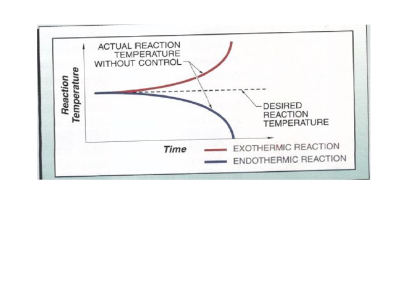
Слайд 7Process dynamics
The degree of difficulty of controlling a process depends on
the characteristics of the process variable, the selected control variable, and the process itself. Control systems must be designed to work with the process dynamics to produce the best control.
Process dynamics are the attributes of a process that describe how a process responds to load changes imposed upon it. These three attributes are gain, dead time, lags.
A load change is a change in process operating conditions that changes the process variable and must be compensated for by a change in the control variable. In most process, a load changes is a change in the amount of material being handled, but it can also be changes in temperature or pressure of process feed streams or energy sources.

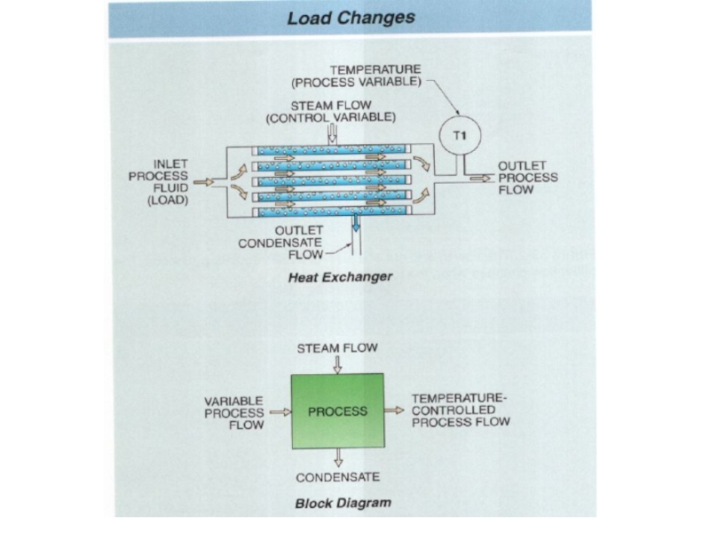
Слайд 9Process Gain
Gain is a ratio of the change in output to
the charge in input of a process. Gain can be measured using any unit.
An example gain is heating a process fluid with steam in a heat exchanger. The gain is the change in temperature of a process fluid through a heat exchanger due to a change in the steam flow rate through the other side of the heat exchanger. For example, heat exchanger is used to raise the temperature of a process fluid from 95° F (T1) to 105° F (T2) by increasing the flow of steam from 380 lb/hr (F1) to 500 lb/hr (F2). The gain is calculated as follows:
An example gain is heating a process fluid with steam in a heat exchanger. The gain is the change in temperature of a process fluid through a heat exchanger due to a change in the steam flow rate through the other side of the heat exchanger. For example, heat exchanger is used to raise the temperature of a process fluid from 95° F (T1) to 105° F (T2) by increasing the flow of steam from 380 lb/hr (F1) to 500 lb/hr (F2). The gain is calculated as follows:

Слайд 10Lags
A lag is a delay in the response of a
process that represents the time it takes for a process to respond completely when there is a change in inputs to the process. A lag is caused by capacitance and resistance. Capacitance is the ability of a process to store material or energy. Capacitance is present in process with storage tanks, surge tanks, or piping systems with a large volume. Resistance is an opposition to the potential that moves material or energy in or out of a process. Resistance is commonly seen as the resistance to flow through ducts, pipes, and fittings. Potential is a driving force that causes material or energy to move through a process. Potential may be fluid pressure, temperature difference, or electrical voltage.
The combination of a single capacitance and resistance results in the formation of a lag with a single time constant. A lag in a process with a single time constant has the same properties as a lag produced by a combination of resistance and capacity
The combination of a single capacitance and resistance results in the formation of a lag with a single time constant. A lag in a process with a single time constant has the same properties as a lag produced by a combination of resistance and capacity


Слайд 12Dead time
Dead time is the period of time that occurs
between the time change is made to a process and the time the first response to that change is detected.
An example is temperature measurement in a pipe when the sensor is significant distance downstream from a heat exchanger.
An example is temperature measurement in a pipe when the sensor is significant distance downstream from a heat exchanger.

Слайд 13Control functions
Controllers are made up of various functions, such as adjustable
setpoints, setpoint tracking, manual output, and bumpless transfer. Most of these functions are also available in pneumatic or electronic controllers, but may take different forms.
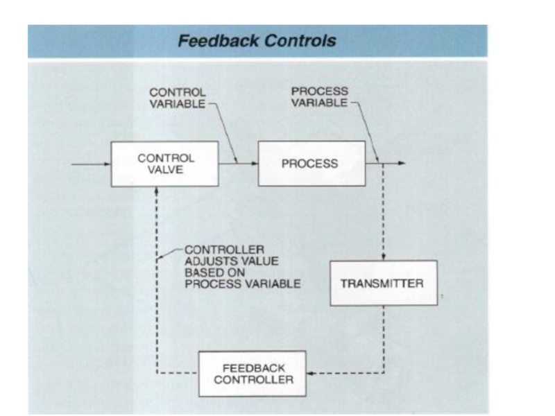
A setpoint (SP) is the desired value at which a process should be controlled and is used by comparison with the process variable.
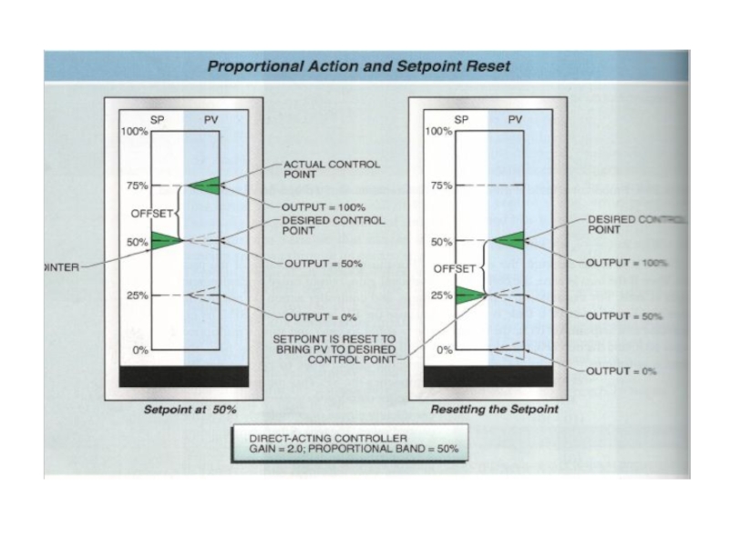
Error is the difference between a process variable and a setpoint. The use of error doesn’t imply that there is a mistake or inaccuracy in measurement. It simply means difference between PV and SP.
Offset is a steady –state error that is permanent part of system. Offset has occasionally been used instead of error to describe the diiference between the PV and SP.
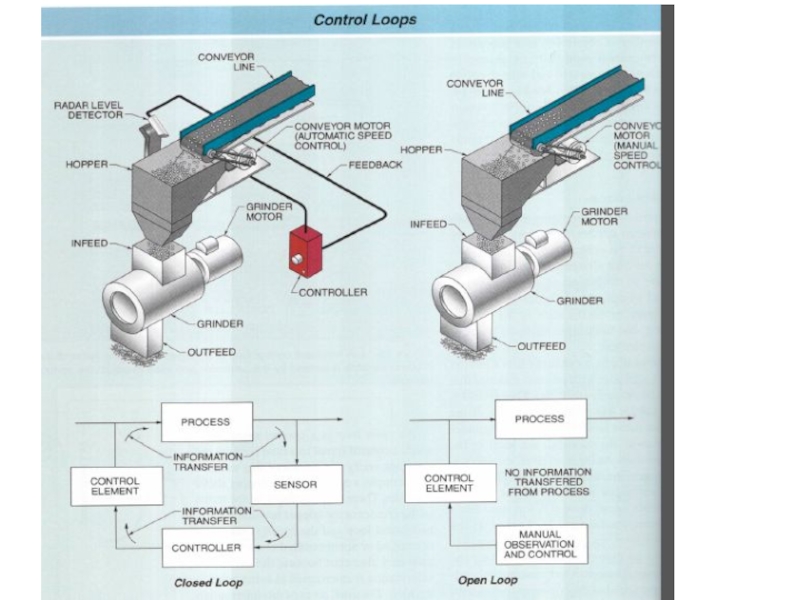
Feedback is a control design used where a controller is connected to a process in an arrangement such that any change in the process is measured and used to adjust action by controller.
A setpoint (SP) is the desired value at which a process should be controlled and is used by comparison with the process variable.
Error is the difference between a process variable and a setpoint. The use of error doesn’t imply that there is a mistake or inaccuracy in measurement. It simply means difference between PV and SP.
Offset is a steady –state error that is permanent part of system. Offset has occasionally been used instead of error to describe the diiference between the PV and SP.
Feedback is a control design used where a controller is connected to a process in an arrangement such that any change in the process is measured and used to adjust action by controller.

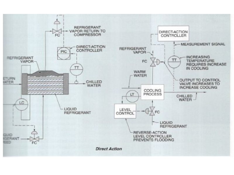
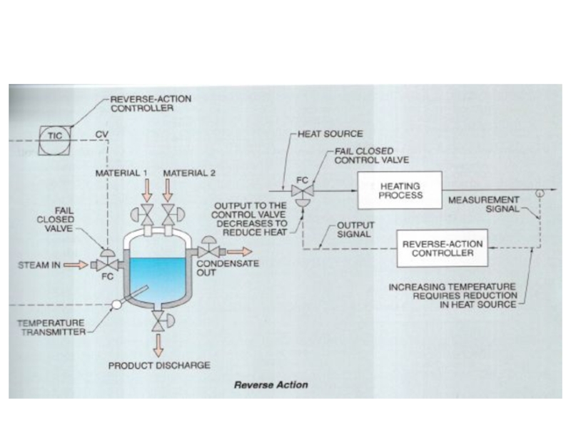
Слайд 16Control actions
Direct action is a form of control action where the
controller output increases with an increase in the measurement of the process variable (PV).
Reverse action is a form of control action where the controller output decreases with an increase in the measurement of the process variable (PV).
Reverse action is a form of control action where the controller output decreases with an increase in the measurement of the process variable (PV).


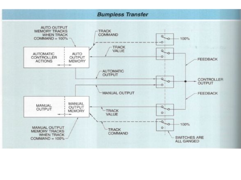
Слайд 21Bumpless transfer
Bumpless transfer is a controller function that eliminates any sudden
change in putput value when the controller is switched from automatic to manual mode or back again. This accomplished by the use of two memory and tracking functions. When in automatic mode, the controller output is fed back to the manual output memory module. Thus manual value tracks the output of the controller. The most modern controllers have a setpoint tracking circuit that makes switching between these modes as simple as selecting the desired mode position. Generally, switching from manual to automatic requires adjusting the setpoint of the controller to actual controlled point (PV) and then switching the mode (alligning the setpoint indicator to the measurement indicator. PV) and other hand switching from automatic to manual may require only a simple repositioning of the mode detector)

Слайд 23Controller Algorithms
The actions of controllers can be divided into groups based
upon the functions of their control mechanism. Each type of controller has advantages and disadvantages and will meet the needs of different
applications. Grouped by control mechanism function, the three types of controllers are:
Discrete controllers
Multistep controllers
Continuous controllers
DISCRETE CONTROLLERS
Discrete controllers are controllers that have only two modes or
positions: on and off.
applications. Grouped by control mechanism function, the three types of controllers are:
Discrete controllers
Multistep controllers
Continuous controllers
DISCRETE CONTROLLERS
Discrete controllers are controllers that have only two modes or
positions: on and off.

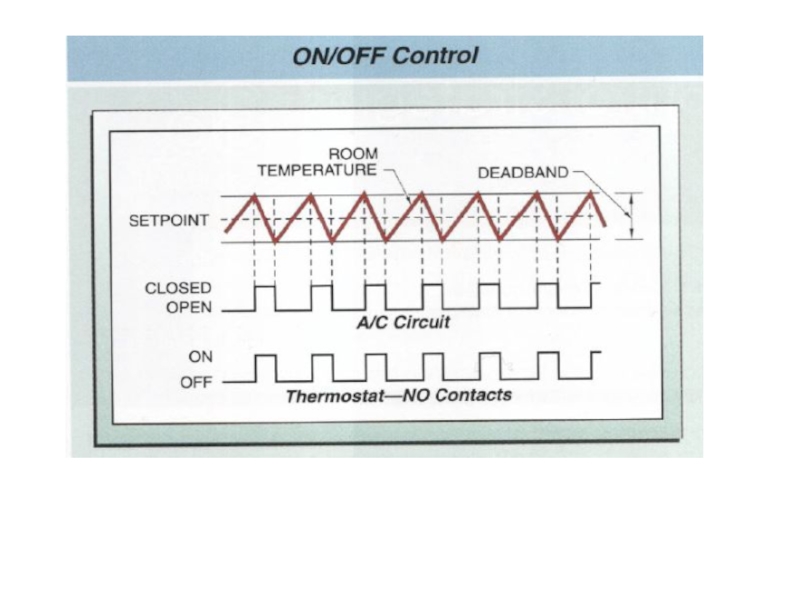
Слайд 24A common example of a discrete controller is a home hot
water heater. When the temperature of the water in the tank falls below setpoint, the burner turns on. When the water in the tank reaches setpoint, the burner turns off. Because the water starts
cooling again when the burner turns off, it is only a matter of time before the cycle begins again. This type of control doesn’t actually hold the variable at setpoint, but keeps the variable within proximity of setpoint in what is known as a dead zone (Figure 7.15).
cooling again when the burner turns off, it is only a matter of time before the cycle begins again. This type of control doesn’t actually hold the variable at setpoint, but keeps the variable within proximity of setpoint in what is known as a dead zone (Figure 7.15).
DISCRETE CONTROLLERS
Common examples of ON/OFF devices
Are air conditioning compressors, electric heating stages gas valves,
refrigeration compressors, and constant speed fans.

Слайд 26MULTISTEP CONTROLLERS
Multistep controllers are controllers that have at least one
other possible position in addition to on and off. Multistep controllers operate similarly to discrete controllers, but as setpoint is approached, the multistep controller takes intermediate steps. Therefore, the oscillation around setpoint can be less dramatic when multistep controllers are employed than when discrete controllers are used
(Figure 7.16).
(Figure 7.16).

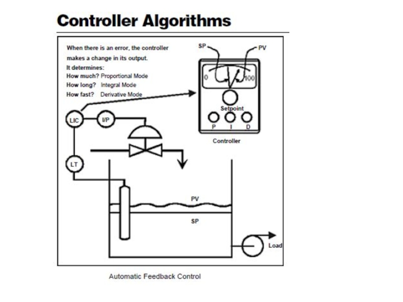
Слайд 27CONTINUOUS CONTROLLERS
Controllers automatically compare the value of the PV to the
SP to
determine if an error exists. If there is an error, the controller adjusts
its output according to the parameters that have been set in the
controller. The tuning parameters essentially determine:
How much correction should be made? The magnitude of the
correction( change in controller output) is determined by the
proportional mode of the controller.
How long should the correction be applied? The duration of the
adjustment to the controller output is determined by the integral mode
of the controller
How fast should the correction be applied? The speed at which a
correction is made is determined by the derivative mode of the
controller.

Слайд 29Why Controllers Need Tuning?
Controllers are tuned in an effort to match
the characteristics of the control equipment to the process so that two goals are achieved: is the foundation of process control measurement in that electricity:
The system responds quickly to errors.
The system remains stable (PV does not oscillate around the SP).
GAIN
Controller tuning is performed to adjust the manner in which a control
valve (or other final control element) responds to a change in error.
In particular, we are interested in adjusting the gain of the controller
such that a change in controller input will result in a change in
Gain is defined simply as the change in output divided by the change
in input.

Слайд 30Examples:
Change in Input to Controller - 10%
Change in Controller Output -
5%
Gain = 5% / 10% = 0.5
Gain = 5% / 10% = 0.5

Слайд 31PROPORTIONAL ACTION
Proportional (P) control is method of changing the output of
a controller by an amount proportional to an error.
The proportional mode is used to set the basic gain value of the
controller. The setting for the proportional mode may be expressed as either:
1. Proportional Gain
2. Proportional Band
In electronic controllers, proportional action is typically expressed as proportional gain. Proportional Gain (Kc) answers the question:
"What is the percentage change of the controller output relative to the
percentage change in controller input?"
Proportional Gain is expressed as:
Gain, (Kc) = ∆Output% / ∆ Input %
 control is method of changing the output of a controller by an")
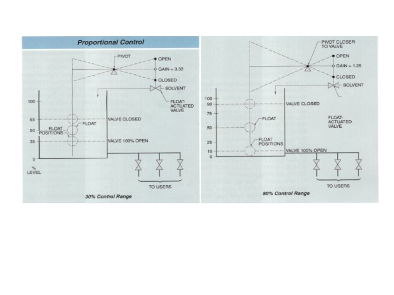
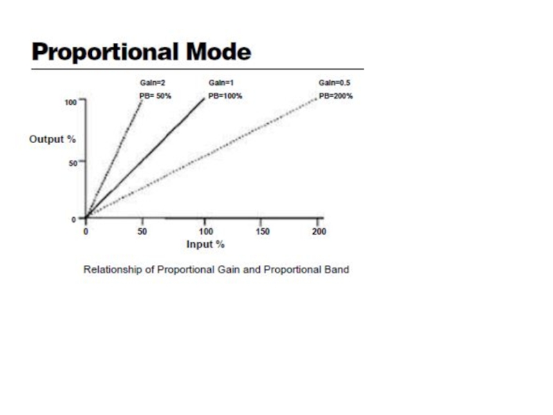
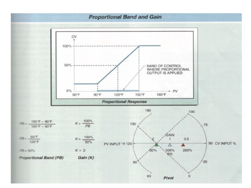
Слайд 33PROPORTIONAL BAND
Proportional Band (PB) is another way of representing the same
information
and answers this question:
"What percentage of change of the controller input span will cause a
100% change in controller output?“
Proportional band is the range of input values that corresponds to a full range of output from a controller, stated as a percentage.
PB = ∆ Input (% Span) For 100% ∆ Output
PB = control range/process range
Converting Between PB and Gain
PB = 100/Gain
Gain = 100%/PB
 is another way of representing the sameinformation and answers this question:")
Слайд 38
Proportional, Derivative Control
The stability and overshoot problems that arise when a
proportional controller is used at high gain can be mitigated by adding a term proportional to the time-derivative of the error signal. The value of the damping can be adjusted to achieve a critically damped response.

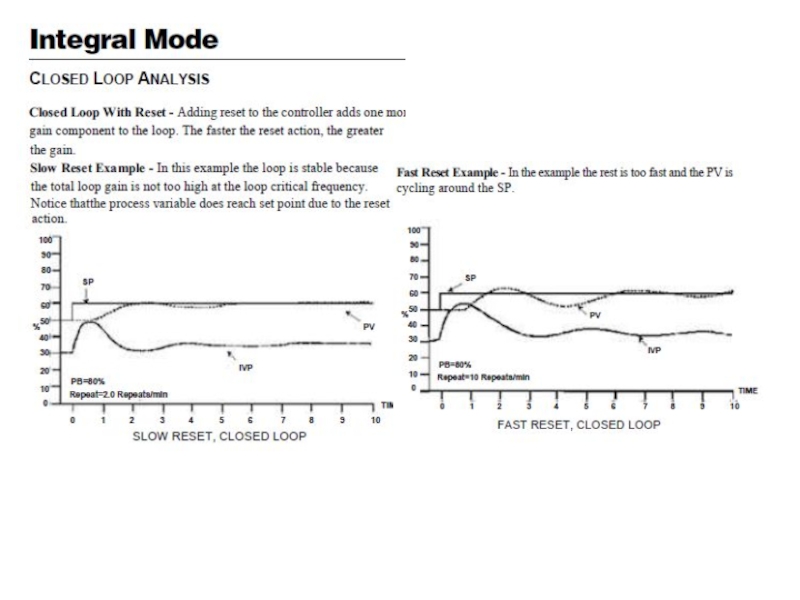
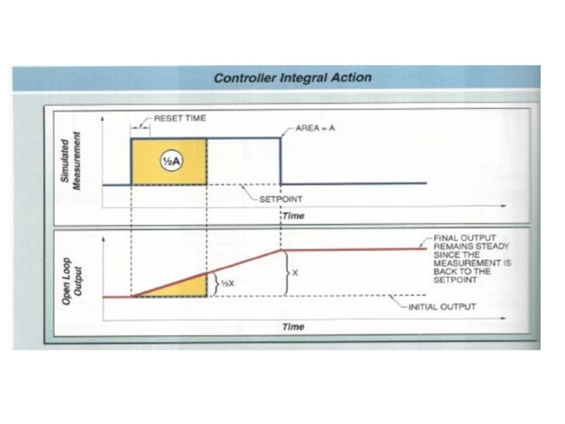
Слайд 39INTEGRAL (I) CONTROL (RESET)
Duration of Error and Integral Mode - Another
component of error is the duration of the error, i.e., how long has the error existed? The controller output from the integral or reset mode is a function of the duration of the error. Integral control is a method of changing the output of a controller by an amount proportional to an error and the duration of that error. The mathematical function of integration is the summtion of the error over a period of time.
Purpose- The purpose of integral action is to return the PV to SP. This is
accomplished by repeating the action of the proportional mode as long as an error exists. With the exception of some electronic controllers, the integral or reset mode is always used with the proportional mode.
Purpose- The purpose of integral action is to return the PV to SP. This is
accomplished by repeating the action of the proportional mode as long as an error exists. With the exception of some electronic controllers, the integral or reset mode is always used with the proportional mode.
Setting - Integral, or reset action, may be expressed in terms of:
Reset rate - How many times the proportional action is repeated each minute (Repeats Per Minute)
Integral time or Reset time - How many minutes are required for 1 repeat to occur. (Minutes Per Repeat)
 CONTROL (RESET)Duration of Error and Integral Mode - Another component of error is")
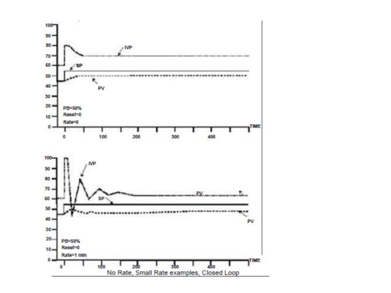
Слайд 42DERIVATIVE CONTROL
Derivative Mode Basics - Some large and/or slow process do
not respond well to small changes in controller output. For example, a large liquid level process or a large thermal process (a heat exchanger) may react very slowly to a small change in controller output. To improve response, a large initial change in controller output may be applied. This action is the role of the
derivative mode.
The Derivative setting is expressed in terms of minutes. In operation, the controller first compares the current PV with the last value of the PV. If there is a change in the slope of the PV, the controller determines what its output would be at a future point in time (the future point in time is determined by the value of the derivative setting, in minutes). The derivative mode immediately increases the output by that amount.

Слайд 43Derivative Mode
Example - Let's start a closed loop example by looking
at a temperature control system. IN this example, the time scale has been lengthened to help illustrate controller actions in a slow process. Assume a proportional band setting of 50%. There is no reset at this time. The proportional gain of 2 acting on a 10% change in set point results in a change in controller output of 20%. Because temperature is a slow process the setting time after a change in error is quite long. And, in this example, the PV never becomes equal to the SP because there is no reset
Rate Effect - To illustrate the effect of rate action, we will add the are mode with a setting of 1 minute. Notice the very large controller output at time 0. The output spike is the result of rate action. Recall
Assume a proportional band settingof 50%. There is no reset at this time. The proportional gain of 2 acting on a 10% change in set pint results in a change in controller output of 20%. Because temperature is a slow process the setting time after a change in error is quite long. And, in this example, the PV never becomes equal to the SP because there is no reset. that the change in output due to rate action is a function of the speed (rate) of change of error, which in a step is nearly infinite. The addition of rate alone will not cause the process variable to match the
set point.

Слайд 45Proportional+Integral+Derivative Control
Although PD control deals neatly with the overshoot and ringing
problems associated with proportional control it does not cure the problem with the steady-state error. Fortunately it is possible to eliminate this while using relatively low gain by adding an integral term to the control function which becomes

Слайд 46The Characteristics of P, I, and D controllers
A proportional controller (Kp)
will have the effect of reducing the rise time and will reduce, but never eliminate, the steady-state error.
An integral control (Ki) will have the effect of eliminating the steady-state error, but it may make the transient response worse.
A derivative control (Kd) will have the effect of increasing the stability of the system, reducing the overshoot, and improving the transient response.
An integral control (Ki) will have the effect of eliminating the steady-state error, but it may make the transient response worse.
A derivative control (Kd) will have the effect of increasing the stability of the system, reducing the overshoot, and improving the transient response.
 will have the effect")
Слайд 47Proportional Control
By only employing proportional control, a steady state error occurs.
Proportional
and Integral Control
The response becomes more oscillatory and needs longer to settle, the error disappears.
Proportional, Integral and Derivative Control
All design specifications can be reached.
The response becomes more oscillatory and needs longer to settle, the error disappears.
Proportional, Integral and Derivative Control
All design specifications can be reached.


Слайд 49Tips for Designing a PID Controller
1. Obtain an open-loop response and determine
what needs to be improved
2. Add a proportional control to improve the rise time
3. Add a derivative control to improve the overshoot
4. Add an integral control to eliminate the steady-state error
Adjust each of Kp, Ki, and Kd until you obtain a desired overall response.
Lastly, please keep in mind that you do not need to implement all three controllers (proportional, derivative, and integral) into a single system, if not necessary. For example, if a PI controller gives a good enough response (like the above example), then you don't need to implement derivative controller to the system. Keep the controller as simple as possible.

Слайд 50Not every process requires a full PID control strategy. If a
small offset
has no impact on the process, then proportional control alone may be
sufficient.
PI control is used where no offset can be tolerated, where noise
(temporary error readings that do not reflect the true process variable
condition) may be present, and where excessive dead time (time after
a disturbance before control action takes place) is not a problem.
In processes where no offset can be tolerated, no noise is present, and
where dead time is an issue, customers can use full PID control.
Proportional, PI, and PID Control

Слайд 51
By using all three control algorithms together, process operators can:
Achieve rapid response to major disturbances with derivative control
Hold the process near setpoint without major fluctuations with proportional control
Eliminate offset with integral control
Hold the process near setpoint without major fluctuations with proportional control
Eliminate offset with integral control

Слайд 52Cascade (Remote Setpoint controllers)
Cascade control is a control strategy where a
primary controller, which controls the ultimate measurement, adjusts the setpoint of a secondary controller. The primary objective in cascade control is to divide a control process into two portions , where a secondary control loop is formed a major disturbance. There are two important reasons for using a cascade loop:
Better control
Reduced lag times
Better control
Reduced lag times
Cascade control is a control strategy where a primary controller, which controls")
Слайд 53Ratio control
Ratio control loops are designed to ratio (or proportion) the
rates of flow between two separate flows entering a mixing point. The ratio controller is designed so that its output represents the exact flow rate needed by the controlled flow loop to remain in allignment with the desired ratio to the uncontrolled flow.
 the rates of flow between")
Слайд 54Feedforward control
Feedforward control is a control strategy that only controls
the inputs to a process without feedback from the output of the process. Theoritically, by knowing and controlling all the properties of a process, a feedforward controller can produce a product satisfying all requirements. Feedforward control systems have an advantage over feedback control systems in that they are designed to compensate for any disturbances before they affect the product. If frequent load changes occur in a process and a feedback controller cannot manage the changes, a feedforward system can be added to a regulate a product stream before it enters a process.

Слайд 55Digital controllers
A digital controller is a controller that uses microprocessor technology
and special programming to perform the controller function. Instead of mechanical linkages, pneumatic pressures or electronic circuits, a digital controller uses mathematical equation. Analog inputs are converted to digital numbers that are processed by the controller equations and then converted back to analog output.
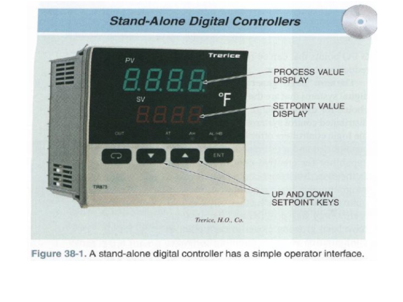
Stand –Alone Digital Controllers
A stand-alone digital controller is general type of the microprocessor-based controller with all required operating components enclosed in housing.
Stand alone controllers usually have only one controller function and one output, but may have two or more. The inputs usually accept any type of signal, but may not provide DC power for a transmitter.

Слайд 57Direct Computer Control System
A direct computer control system is a control
system that uses a computer as the controller. The development of more robust and secure personal computer software, which has a true interruptible operating system strategy, has led to a greater acceptance of this arrangement for process control.
There are also separate control and display software systems that allow the user to develop the desired control strategies
There are also separate control and display software systems that allow the user to develop the desired control strategies

Слайд 58Distributed Control Systems (DCS)
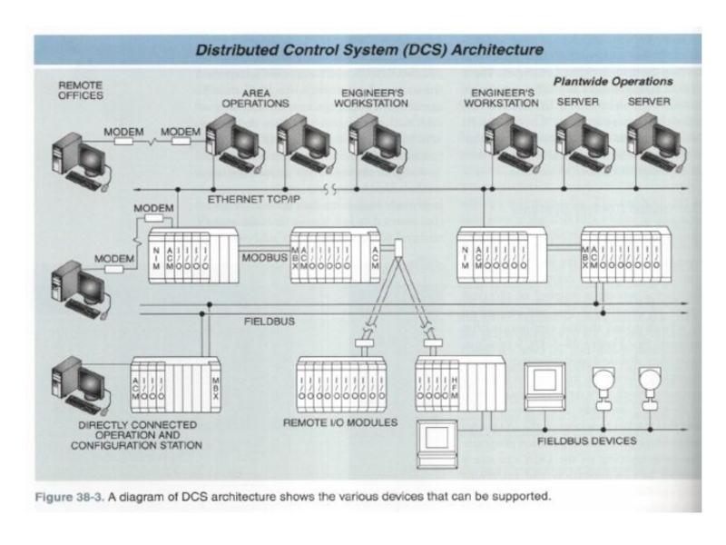
A distributed control systems is a control system
where the individual functions that make up a control system are distributed among a number of physical pieces of equipment that are connected by a high-speed digital communication network. DCS systems since they are designed to control slow changing chemical and petrochemical processes, work very well with scan speed of about 0.5 seconds.
The distributed units that house the various functions are usually rack mounted in cabinets. The main units consist of dual 24VDC power supplies, analog input modules, discrete input modules, analog, output discrete output modules and controller modules.
Information from the input modules is made available to the high speed communication network to be used by any device or program in the system. A number of digital signals such as Ethernet, RS 232, Modbus and so on, can be imported from special controllers like PLC and PC systems.
A distributed control systems is a control system where the individual functions")
Слайд 60Programmable Logic Controller (PLC)
A programmable logic controller is a control system
with an architecture very to similar to that of a DCS, with self-contained power supplies, distributed inputs and outputs, and a controller module, all connected on high-speed digital communication networks. A PLC is designed to be more rugged than DCS , since PLCs were originally designed fore mounting on the production floor in discrete manufacturing areas.
Most PlCs are programmed using a ladder logic format, but some of newer large systems can use other programming methods. Typically there is no data storage capability available in these systems. However, they can pass information to a conventional PC where it can be stored.
Most PlCs are programmed using a ladder logic format, but some of newer large systems can use other programming methods. Typically there is no data storage capability available in these systems. However, they can pass information to a conventional PC where it can be stored.
A programmable logic controller is a control system with an architecture very")
Слайд 61Automatic control system
In the control method of the automated control
systems (ACS) are divided into non-adaptive (or unadaptable) and
adaptive (or adapting) system.
adaptive (or adapting) system.
Non-adaptive automatic control systems do not adapt to the changing conditions of the control object. This is the most simple system without changing its structure and parameters of the control process. Almost all of the automated control system refer to adaptive ACS. For these systems, based on a priori (before the start of the current) information for the design and setup of choosing the structure and parameters, which provide the desired properties of the system (performance management purposes) for typical or the most likely conditions for its operation (if necessary, you can manually rebuild the system).
 are divided")
Слайд 62Adaptive ACS
Adaptive ACS - these are systems in which the
parameters of the control devices or control algorithms automatically and purposefully altered for optimal control of the object, and the characteristics of the object or external influence on it can be changed in advance in an unforeseen way. Adaptive ACS able to change the structure, settings, or program their actions in the management process. As in the management process is an automatic change of parameters or structure of the system, the adaptive automatic control system is also called a self-adjusting. Adaptive ACS is divided into two types: extreme system that will automatically find the extremum of the controlled quantity, as well as his position is changed during operation of the object, the system automatically changes the search direction, speed, etc. (Changes the program of its actions); optimalpl systems, which are used in order to obtain the optimum conditions of the object, characterized extremum control criterion under certain restrictions.