- Главная
- Разное
- Дизайн
- Бизнес и предпринимательство
- Аналитика
- Образование
- Развлечения
- Красота и здоровье
- Финансы
- Государство
- Путешествия
- Спорт
- Недвижимость
- Армия
- Графика
- Культурология
- Еда и кулинария
- Лингвистика
- Английский язык
- Астрономия
- Алгебра
- Биология
- География
- Детские презентации
- Информатика
- История
- Литература
- Маркетинг
- Математика
- Медицина
- Менеджмент
- Музыка
- МХК
- Немецкий язык
- ОБЖ
- Обществознание
- Окружающий мир
- Педагогика
- Русский язык
- Технология
- Физика
- Философия
- Химия
- Шаблоны, картинки для презентаций
- Экология
- Экономика
- Юриспруденция
Influence of supply voltage on torque–speed curve презентация
Содержание
- 1. Influence of supply voltage on torque–speed curve
- 3. Table of synchronous speed of rotation of
- 4. Influence of supply voltage on torque–speed curve
- 5. To illustrate the problem, consider the torque–speed
- 6. Now suppose that the voltage falls to
- 7. The drop in speed from 95% of
- 8. Speed control We have seen that to
- 9. Pole-changing motors For some applications continuous speed
- 10. It was soon realised that if half
- 11. It was not until the advent of
- 12. The beauty of the PAM method is
- 13. Voltage control of high-resistance cage motors Where
- 14. But if special high-rotor resistance motors are
- 15. Voltage control became feasible only when relatively
- 16. Speed control of wound-rotor motors The fact
- 17. Torque–speed characteristics – constant v/f operation When
- 18. As expected, the no-load speeds are directly
- 19. We also note that the pull-out torque
- 20. The low-frequency performance can be improved by
- 21. The curves in Figure have an obvious
- 22. We should note that the availability of
- 23. Beyond the base frequency, the V/f ratio
- 24. Modelling the electromechanical energy conversion process The
- 25. A very important observation in relation to
- 26. Hence if we build from the exact
- 27. At any given slip, the power delivered
- 28. Firstly, given the complexity of the spatial
- 29. The key to developing the representation lies
- 30. In the supply-frequency equivalent circuit, e.g. Figure,
- 31. Limitations imposed by the inverter – constant
- 32. The current limit feature imposes an upper
- 33. In the region below base speed, the
- 34. At the upper limit of the constant
- 35. Generating and braking Having explored the torque–speed
- 40. We can see from Figure that the
- 42. Injection braking This is the most widely
- 43. A typical torque–speed curve for braking a
- 44. This is in line with what we
- 45. Plug reversal and plug braking Because the
- 46. The motor is initially assumed to be
- 47. The speed–time curve is shown in Figure
- 48. Very rapid reversal is possible using plugging;
- 49. We should note that, whereas, in the
- 50. Stepping motors Stepping motors are attractive because
- 51. Performance Features of MOONS' Stepping Motors
- 52. • Forward & Reverse, Pause and Holding
- 53. Basic Structure and Motor Operation
- 54. A basic stepping motor system is shown
- 55. This one to one correspondence between pulses
- 56. Technical Data and Terminology • Load Calculations
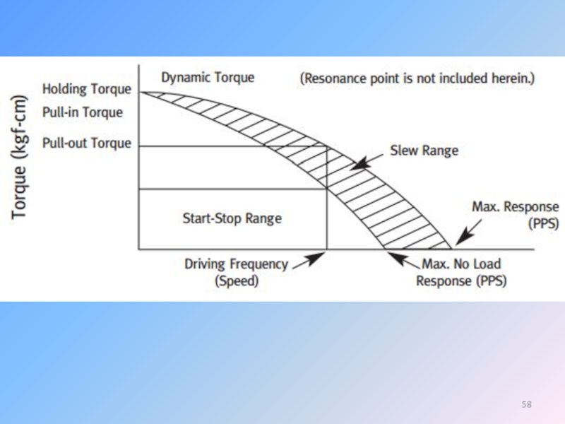
- 57. • Speed-Torque Characteristics The dynamic torque
- 59. Борьба с нежелательными явлениями
- 60. 2. Start/Stop region: the region in which
- 61. 7. Pull-in Torque: the maximum dynamic torque
- 62. 10. Accuracy: This is defined as the
- 63. 11. Hysteresis Error This is the maximum
- 64. 12. Resonance: A step motor operates on
- 65. Динамические характеристики Динамическими характеристиками называются
- 66. Динамические характеристики: 1 - удерживающий момент;
- 67. Максимальный статический эффект имеет сразу два
- 68. «Мертвые» положения ротора Существует
- 69. Во всех случаях, когда рассчитывается либо
- 70. Максимальная частота приемистости определяется как максимальная
- 71. Principle of motor operation The principle on
- 72. Before exploring constructional details, it is worth
- 73. The answer is that in the vast
- 74. As mentioned above, reluctance torque originates in
- 75. All the torque is then produced by
- 76. Because the two torque-producing mechanisms appear to
- 77. The two most important types of stepping
- 78. Motor characteristics Static torque–displacement curves From
- 79. We now turn to a typical static
- 80. Typical static torque–displacement curves for a 3-phase
- 81. There are three curves, one for each
- 82. When only one phase, say A, is
- 83. There are also four unstable equilibrium positions,
- 84. The characteristic of static (holding) torque -
- 85. Step position error and holding torque In
- 86. The true step position is at the
- 87. The existence of a step position error
- 88. As long as the load torque is
- 89. The static load angle is defined as,
- 90. Step response It was pointed out earlier
- 91. Knowing , we can
- 92. Two remedies are available, the simplest being

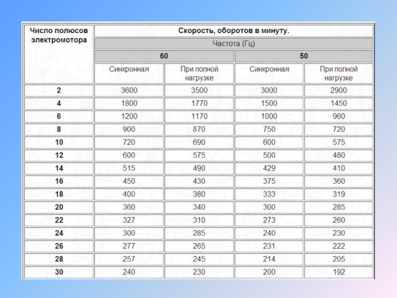
Слайд 3Table of synchronous speed of rotation of induction motors as a
Rotational speed of induction motor, rev/min
number of pole pairs
Frequ-
ency, Hz

Слайд 4Influence of supply voltage on torque–speed curve
We established earlier that at

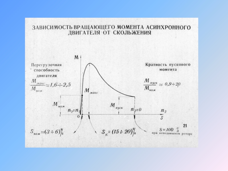
Слайд 5 To illustrate the problem, consider the torque–speed curves for a cage

Слайд 6 Now suppose that the voltage falls to 90%. The load torque

Слайд 7 The drop in speed from 95% of synchronous to 94% may
The stator current will also be above rated value, so if the motor is allowed to run continuously, it will overheat. This is one reason why all large motors are fitted with protection, which is triggered by over temperature. Many small and medium motors do not have such protection, so it is important to guard against the possibility of under voltage operation.

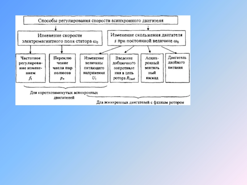
Слайд 8Speed control
We have seen that to operate efficiently an induction motor
The pole number has to be an even integer, so where continuously adjustable speed control over a wide range is called for, the best approach is to provide a variable-frequency supply. In this chapter we are concerned with constant frequency mains operation, so we have a choice between pole-changing, which can provide discrete speeds only, or slip control which can provide continuous speed control, but is inherently inefficient.

Слайд 9Pole-changing motors
For some applications continuous speed control may be an unnecessary
Previously we established that the pole number of the Weld was determined by the layout and interconnection of the stator coils, and that once the winding has been designed, and the frequency specified, the synchronous speed of the Weld is fixed. If we wanted to make a motor, that could run at either of two different speeds, we could construct it with two separate stator windings (say 4-pole and 6-pole), and energise the appropriate one. There is no need to change the cage rotor since the pattern of induced currents can readily adapt to suit the stator pole number. Early 2-speed motors did have 2 distinct stator windings, but were bulky and inefficient.

Слайд 10 It was soon realised that if half of the phase belts

Слайд 11 It was not until the advent of the more sophisticated pole
 method")
Слайд 12 The beauty of the PAM method is that it is not

Слайд 13Voltage control of high-resistance cage motors
Where efficiency is not of paramount

Слайд 14 But if special high-rotor resistance motors are used, the slope of
The most unattractive feature of this method is the low efficiency, which is inherent in any form of slip control. fierecall that the rotor efficiency at slip s is
( ), so if we run at say 70% of synchronous speed (i.e. s = 0.3), 30% of the power crossing the air-gap is wasted as heat in the rotor conductors. The approach is therefore only practicable where the load torque is low at low speeds, so that at high slips the heat in the rotor is tolerable. A fan-type characteristic is suitable, as shown in Figure, and many ventilating systems therefore use voltage control.

Слайд 15 Voltage control became feasible only when relatively cheap thyristor a.c. voltage
Applications are numerous, mainly in the range 0.5–10 kW, with most motor manufacturers offering high-resistance motors specifically for use with thyristor regulators.

Слайд 16Speed control of wound-rotor motors
The fact that the rotor resistance can
A set of torque–speed characteristics is shown in Figure, from which it should be clear that by appropriate selection of the rotor circuit resistance, any torque up to typically 1.5 times full-load torque can be achieved at any speed.

Слайд 17Torque–speed characteristics – constant v/f operation
When the voltage at each frequency

Слайд 18 As expected, the no-load speeds are directly proportional to the frequency,

Слайд 19 We also note that the pull-out torque and the torque stiffness

Слайд 20 The low-frequency performance can be improved by increasing the V/f ratio

Слайд 21 The curves in Figure have an obvious appeal because they indicate
This region of the characteristics is known as the ‘constant torque’ region, which means that for frequencies up to base speed, the maximum possible torque which the motor can deliver is independent of the set speed. Continuous operation at peak torque will not be allowable because the motor will overheat, so an upper limit will be imposed by the controller, as discussed shortly. With this imposed limit, operation below base speed corresponds to the armature-voltage control region of a d.c. drive, as exemplified in Figure

Слайд 22 We should note that the availability of high torque at low

Слайд 23 Beyond the base frequency, the V/f ratio reduces because V remains
Although the curves in Figure show what torque the motor can produce for each frequency and speed, they give no indication of whether continuous operation is possible at each point, yet this matter is of course extremely important from the user’s viewpoint, and is discussed next.

Слайд 24Modelling the electromechanical energy conversion process
The behaviour of the motor was

Слайд 25 A very important observation in relation to what we are now

Слайд 26 Hence if we build from the exact transformer circuit, we obtain
‘Exact’ per-phase equivalent circuit of induction motor.
The secondary (rotor) parameters have been referred to the primary (stator) side

Слайд 27 At any given slip, the power delivered to this ‘load’ resistance
We will see how to use the equivalent circuit to predict and illuminate motor behaviour in the next section, but first there are two points worth making.

Слайд 28 Firstly, given the complexity of the spatial and temporal interactions in
Secondly, the following brief discussion is offered for the benefit of readers who are seeking at least some justification for introducing the fictitious resistance , though it has to be admitted that full treatment is beyond our scope.

Слайд 29 The key to developing the representation lies in ensuring that the
at frequency , where is the e.m.f. induced under locked rotor (s = 1) conditions, when the rotor frequency is the same as the supply frequency, i.e. f. This e.m.f. acts on the series combination of the rotor resistance and the rotor leakage reactance, which at frequency is given by , where is the rotor leakage reactance at supply frequency. Hence the magnitude of the rotor current is given by

Слайд 30 In the supply-frequency equivalent circuit, e.g. Figure,
the secondary e.m.f. is
we require the slip-frequency rotor resistance and reactance to be divided by s, in which case the secondary current would be correctly given by

Слайд 31Limitations imposed by the inverter – constant power and constant torque
The main concern in the inverter is to limit the currents to a safe value as far as the main switching devices are concerned. The current limit will be at least equal to the rated current of the motor, and the inverter control circuits will be arranged so that no matter what the user does the output current cannot exceed a safe value.

Слайд 32 The current limit feature imposes an upper limit on the permissible

Слайд 33 In the region below base speed, the motor can therefore develop
Above base speed of the flux is reduced inversely with the frequency; because the stator (and therefore rotor) currents are limited, the maximum permissible torque also reduces inversely with the speed, as shown in Figure. This region is therefore known as the ‘constant power’ region. There is of course a close parallel with the d.c. drive here, both systems operating with reduced or weak Weld in the constant power region. The region of constant power normally extends to somewhere around twice base speed, and because the flux is reduced the motor has to operate with higher slips than below base speed to develop the full rotor current and torque.

Слайд 34 At the upper limit of the constant power region, the current

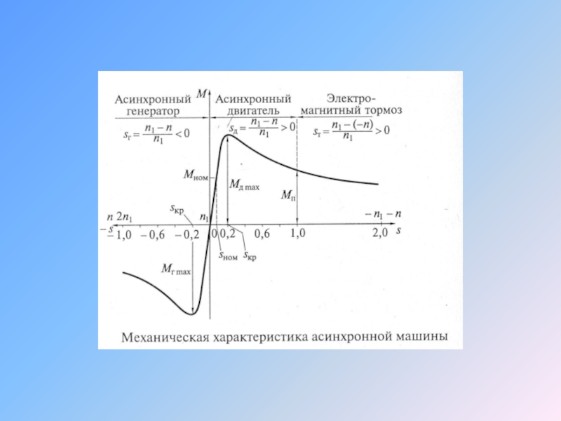
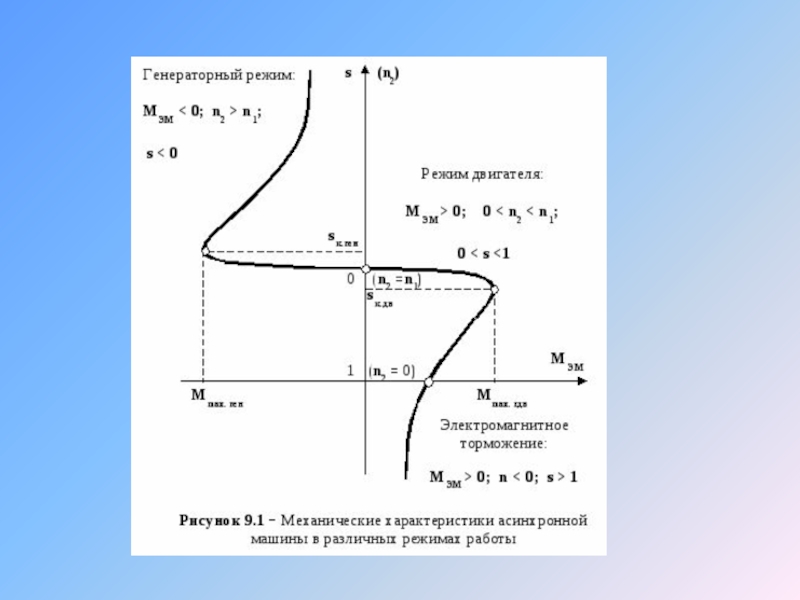
Слайд 35Generating and braking
Having explored the torque–speed curve for the normal motoring
A typical torque–speed curve for a cage motor covering the full range of speeds, which are likely to be encountered in practice, is shown in Figure


Слайд 40 We can see from Figure that the decisive [diˈsīsiv] factor as

Слайд 42Injection braking
This is the most widely used method of electrical braking.
We saw earlier that the speed of rotation of the air-gap Weld is directly proportional to the supply frequency, so it should be clear that since d.c. is effectively zero frequency, the air-gap Weld will be stationary. We also saw that the rotor always tries to run at the same speed as the Weld. So, if the Weld is stationary, and the rotor is not, a braking torque will be exerted.

Слайд 43 A typical torque–speed curve for braking a cage motor is shown

Слайд 44 This is in line with what we would expect, since there

Слайд 45Plug reversal and plug braking
Because the rotor always tries to catch

Слайд 46 The motor is initially assumed to be running light (and therefore
Two of the supply leads are then reversed, thereby reversing the direction of the Weld, and bringing the mirror-image torque–speed curve shown by the solid line into play. The slip of the motor immediately after reversal is approximately 2, as shown by point B on the solid curve. The torque is thus negative, and the motor decelerates, the speed passing through zero at point C and then rising in the reverse direction before settling at point D, just below the synchronous speed.

Слайд 47 The speed–time curve is shown in Figure
We can see that the

Слайд 48 Very rapid reversal is possible using plugging; for example a 1
Plugging can also be used to stop the rotor quickly, but obviously it is then necessary to disconnect the supply when the rotor comes to rest, otherwise it will run-up to speed in reverse. A shaft-mounted reverserotation detector is therefore used to trip out the reverse contactor when the speed reaches zero.

Слайд 49 We should note that, whereas, in the regenerative mode (discussed in
 the")
Слайд 50Stepping motors
Stepping motors are attractive because they can be controlled directly

Слайд 51Performance Features of MOONS' Stepping Motors
• Accurate Position Control
The
• Precise Motor Speed
Step motor running speed, is exactly determined by the frequency of the control pulses. Because the speed is very precise and easy to control, step motors are often used where coordinated motion control is needed.

Слайд 52 • Forward & Reverse, Pause and Holding Function
Motor torque and
• Low Speed Operation
Step motors produce a large amount of torque, and are easy to control, at low speeds. This often eliminates the need for speed reduction gearboxes, reduces costs and saves space.
• Long Life
The brushless design of step motors leads to motors with a very long life. Step motor life is usually determined by the life of the bearings.


Слайд 54 A basic stepping motor system is shown in Figure
The drive contains

Слайд 55 This one to one correspondence between pulses and steps is the

Слайд 56Technical Data and Terminology
• Load Calculations
Torque load (Tf)
Tf =
G: weight
r: radius
B. Inertia load (TJ)
TJ = J * dw/dt
J = M * (R12+R22 ) / 2 (Kg * cm)
M: mass
R1: outside radius
R2: inside radius
dw/dt: angle acceleration
 Tf = G * r G:")
Слайд 57• Speed-Torque Characteristics
The dynamic torque curve is an important aspect of
The followings are some keyword explanations.
1. Working frequency point express the stepping motors rotational speed value at this point
n = q * Hz / (360 * D)
n: rev/sec
Hz: the frequency value at this point
D: the subdividing value of motor driver
q: the step angle of stepping motor
E.g.: 1.8° stepping motor, in the condition of I/2 subdividing (each step 0.9°) runs at 500Hz its speed is 1.25r/s.

Слайд 59
Борьба с нежелательными явлениями
Зазор между роторными и статорными зубцами всегда

Слайд 60 2. Start/Stop region: the region in which a stepping motor can
3. Detent Torque: The maximum torque that can be applied to the shaft of a non-energized motor without causing rotation.
4. Speed-Torque Curve: The speed-torque characteristics of a stepping motor are a function of the drive circuit, excitation method and load inertia.
5. Maximum Slew Frequency: The maximum rate at which the step motor will run and remain in synchronism.
6. Maximum Starting Frequency: The maximum pulse rate (frequency) at which an unloaded step motor can start and run without missing steps or stop without missing steps.

Слайд 61 7. Pull-in Torque: the maximum dynamic torque value that a stepping
8. Pull-out Torque: the maximum dynamic torque value that a stepping motor can load at the particular operating frequency point when the motor has been started. Because of the inertia of rotation the Pull-Out. Torque is always larger than the Pull-In Torque.
9. Slewing Range This is the area between the pull-in and pull-out torque curves where a step motor can run without losing step, when the speed is increased or decreased gradually. Motor must be brought up to the slew range with acceleration and deceleration technique known as ramping.

Слайд 62 10. Accuracy: This is defined as the difference between the theoretical

Слайд 63 11. Hysteresis Error This is the maximum accumulated error from theoretical

Слайд 64 12. Resonance: A step motor operates on a series of input

Слайд 65
Динамические характеристики
Динамическими характеристиками называются характеристики двигателя во время движения либо в
Характеристики пускового момента определяются диапазоном значений момента сопротивления нагрузки, в котором двигатель может запускаться и останавливаться без потери шага для различных частот в наборе импульсов (их около 100). Причина, по которой используется слово "диапазон", а не "максимум", заключается в том, что двигатель не способен запускаться или поддерживать нормальное вращение при малых нагрузках сопротивления в определенных диапазонах частот, как показано на рисунке

Слайд 66
Динамические характеристики: 1 - удерживающий момент; 2 - максимальный пусковой момент;
(В некоторой литературе приводится упрощенная характеристика)

Слайд 67
Максимальный статический эффект имеет сразу два положения:
- Удерживающий. Это максимально
- Фиксирующий. Соответственно, это также максимальный статический эффект, который теоретически может быть приложен к валу невозбужденного двигателя без возникновения последующего вращения. Чем удерживающий момент выше, тем ниже вероятность возникновения погрешностей позиционирования, вызываемых непрогнозируемой нагрузкой (отказали конденсаторы для электродвигателей, например). Полный фиксирующий момент возможен только в тех моделях двигателей, в которых используются постоянные магниты.

Слайд 68
«Мертвые» положения ротора
Существует сразу три положения, в которых ротор полностью
- Положение равновесия. В нем происходит полная остановка возбужденного шагового двигателя.
- Фиксация. Также состояние, в котором останавливается ротор. Но используется это понятие только в отношении тех двигателей, у которых в конструкции имеется постоянный магнит.
В современных моделях шаговых двигателей, которые соответствуют всем нормам экологической и энергетической безопасности, при остановке ротора полностью обесточивается и обмотка.

Слайд 69
Во всех случаях, когда рассчитывается либо измеряется пусковой момент, необходимо также
Характеристики выходного момента иначе называются характеристиками в движении. После того, как выбранный двигатель запустился при определенном управлении, обеспечивающем заданный способ возбуждения в пусковом диапазоне, частота импульсов постепенно возрастает. При некоторой частоте двигатель выпадает из синхронизма. Взаимосвязь между моментом сопротивления нагрузки и максимальной частотой импульсов, при которой сохраняется синхронизм, называется выходной характеристикой (рисунок). Кривая выходной характеристики зависит от схемы управления, способа стыковки, измерительных приборов и других условий.

Слайд 70
Максимальная частота приемистости определяется как максимальная управляющая частота, при которой ненагруженный
Максимальная выходная частота вращения определяется как максимальная (шаговая) частота вращения, при которой ненагруженный двигатель может двигаться без пропуска шагов.
Максимальный пусковой момент определяется как максимальный момент сопротивления нагрузки, с которой двигатель может запускаться и сохранять синхронность при наборе импульсов с частотой до 10 Гц.

Слайд 71Principle of motor operation
The principle on which stepping motors are based

Слайд 72 Before exploring constructional details, it is worth saying a little more

Слайд 73 The answer is that in the vast majority of electrical machines,

Слайд 74 As mentioned above, reluctance torque originates in the tendency of an

Слайд 75 All the torque is then produced by reluctance action, because with

Слайд 76 Because the two torque-producing mechanisms appear to be radically different, the

Слайд 77 The two most important types of stepping motor are the variable
 type and")
Слайд 78Motor characteristics
Static torque–displacement curves
From the previous discussion, it should be clear

Слайд 79 We now turn to a typical static torque–displacement curve, and look

Слайд 80 Typical static torque–displacement curves for a 3-phase 30° per step VR
These show the torque that has to be applied to move the rotor away from its aligned position. Because of the rotor–stator symmetry, the magnitude of the restoring torque when the rotor is displaced by a given angle in one direction is the same as the magnitude of the restoring torque when it is displaced by the same angle in the other direction, but of opposite sign.

Слайд 81 There are three curves, one for each of the three phases,

Слайд 82 When only one phase, say A, is energised, the other two

Слайд 83 There are also four unstable equilibrium positions, (at θ = 45°,
")
Слайд 84 The characteristic of static (holding) torque - displacement is best explained
 torque - displacement is best explained using an electro-magnet and")
Слайд 85Step position error and holding torque
In the previous discussion the load
The origin and extent of the step position error can be appreciated with the aid of the typical torque–displacement curve shown in Figure

Слайд 86 The true step position is at the origin in the figure,

Слайд 87 The existence of a step position error is one of the

Слайд 88 As long as the load torque is less than (Figure), a
, a stable rest position is")
Слайд 89 The static load angle is defined as, the angle between the
The static load angle can be calculated using the formula:

Слайд 90Step response
It was pointed out earlier that the single-step response is

Слайд 91 Knowing , we can judge what the oscillatory

Слайд 92 Two remedies are available, the simplest being to Wt a mechanical