Слайд 1State Space Representation of Dynamic Models and the Kalman Filter
Presenter
Charis Christofides
Joint
Vienna Institute/ IMF ICD
Macro-econometric Forecasting and Analysis
JV16.12, L04, Vienna, Austria May 18, 2016
This training material is the property of the International Monetary Fund (IMF) and is intended for use in IMF Institute courses. Any reuse requires the permission of the IMF Institute.
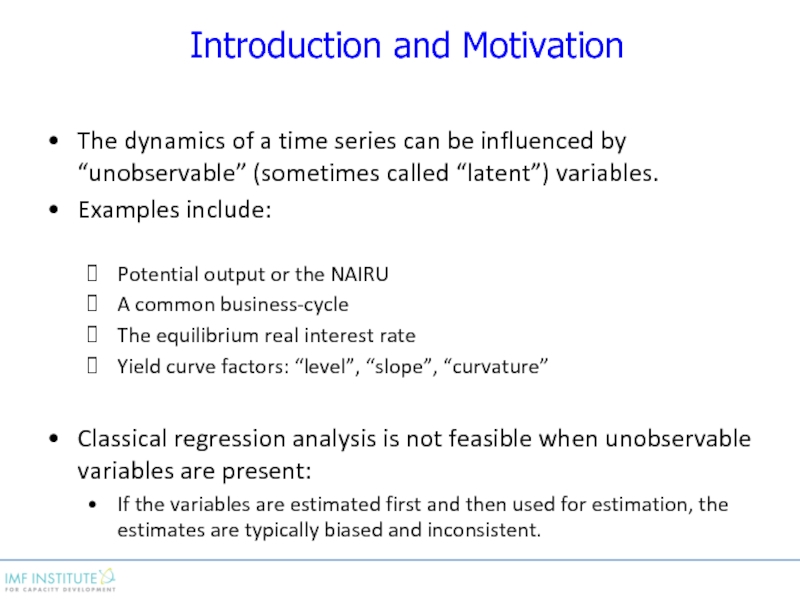
Слайд 2Introduction and Motivation
The dynamics of a time series can be influenced
by “unobservable” (sometimes called “latent”) variables.
Examples include:
Potential output or the NAIRU
A common business-cycle
The equilibrium real interest rate
Yield curve factors: “level”, “slope”, “curvature”
Classical regression analysis is not feasible when unobservable variables are present:
If the variables are estimated first and then used for estimation, the estimates are typically biased and inconsistent.
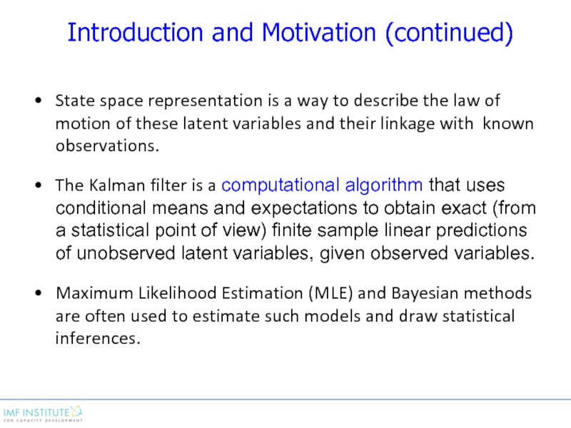
Слайд 3Introduction and Motivation (continued)
State space representation is a way to describe
the law of motion of these latent variables and their linkage with known observations.
The Kalman filter is a computational algorithm that uses conditional means and expectations to obtain exact (from a statistical point of view) finite sample linear predictions of unobserved latent variables, given observed variables.
Maximum Likelihood Estimation (MLE) and Bayesian methods are often used to estimate such models and draw statistical inferences.
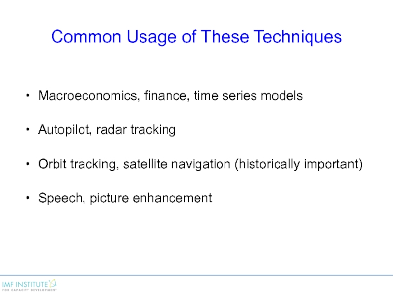
Слайд 4Common Usage of These Techniques
Macroeconomics, finance, time series models
Autopilot, radar tracking
Orbit
tracking, satellite navigation (historically important)
Speech, picture enhancement
Слайд 5Another example
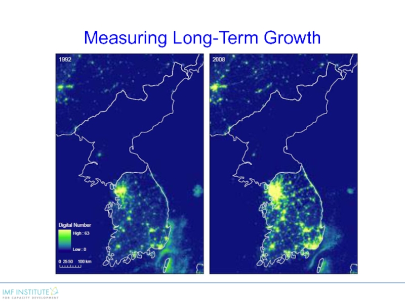
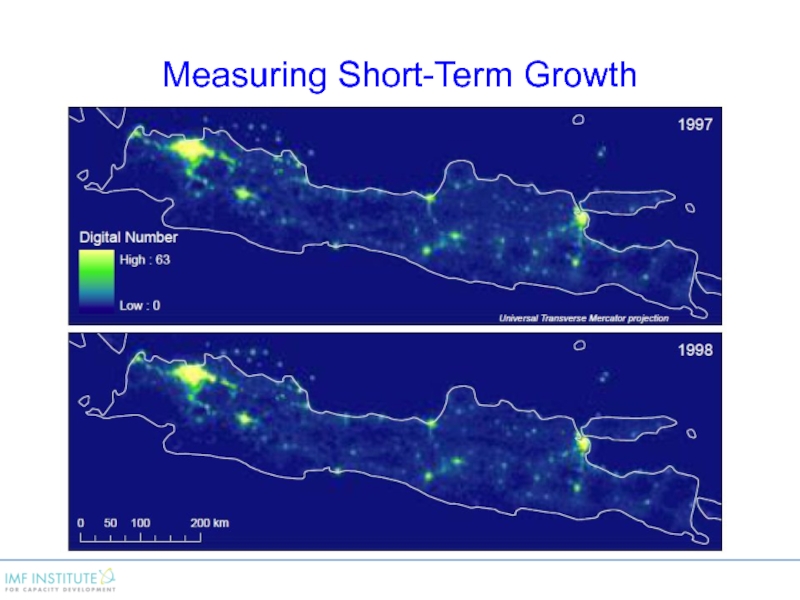
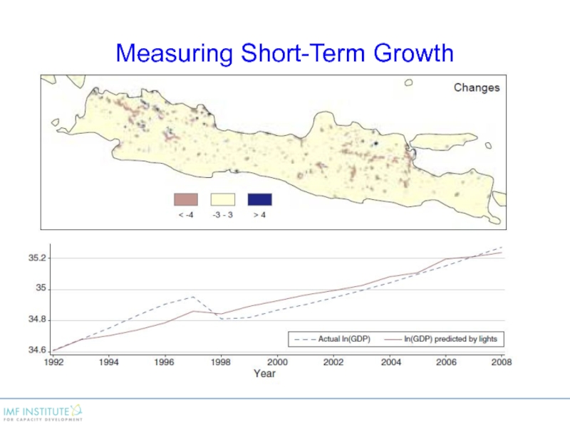
Use nightlight data and the Kalman filter to adjust official
GDP growth statistics.
The idea is that economic activity is closely related to nightlight data.
“Measuring Economic Growth from Outer Space” by Henderson, Storeygard, and Weil AER(2012)
Слайд 9Content Outline: Lecture Segments
State Space Representation
The Kalman Filter
Maximum Likelihood Estimation and
Kalman Smoothing
Слайд 10Content Outline: Workshops
Workshops
Estimation of equilibrium real interest rate, trend growth rate,
and potential output level: Laubach and Williams (ReStat 2003);
Estimation of a term structure model of latent factors: Diebold and Li (J. Econometrics 2006);
Estimation of output gap (various country examples).
Слайд 12Basic Setup
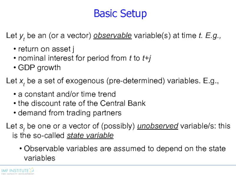
Let yt be an (or a vector) observable variable(s) at
time t. E.g.,
return on asset j
nominal interest for period from t to t+j
GDP growth
Let xt be a set of exogenous (pre-determined) variables. E.g.,
a constant and/or time trend
the discount rate of the Central Bank
demand from trading partners
Let st be one or a vector of (possibly) unobserved variable/s: this is the so-called state variable
Observable variables are assumed to depend on the state variables
Слайд 13Basic Setup
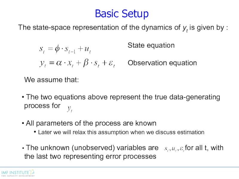
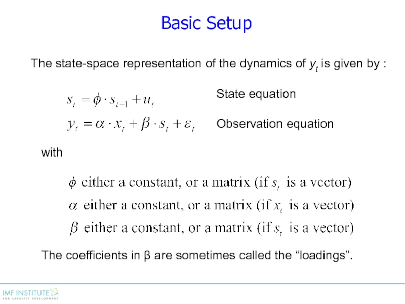
The state-space representation of the dynamics of yt is given
by :
We assume that:
The two equations above represent the true data-generating process for
All parameters of the process are known
Later we will relax this assumption when we discuss estimation
The unknown (unobserved) variables are for all t, with the last two representing error processes
State equation
Observation equation
Слайд 14Basic Setup
The state-space representation of the dynamics of yt is given
by :
with
The coefficients in β are sometimes called the “loadings”.
State equation
Observation equation
Слайд 15Basic Setup
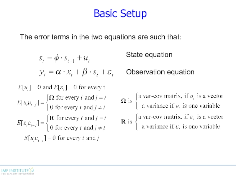
The error terms in the two equations are such that:
State
equation
Observation equation
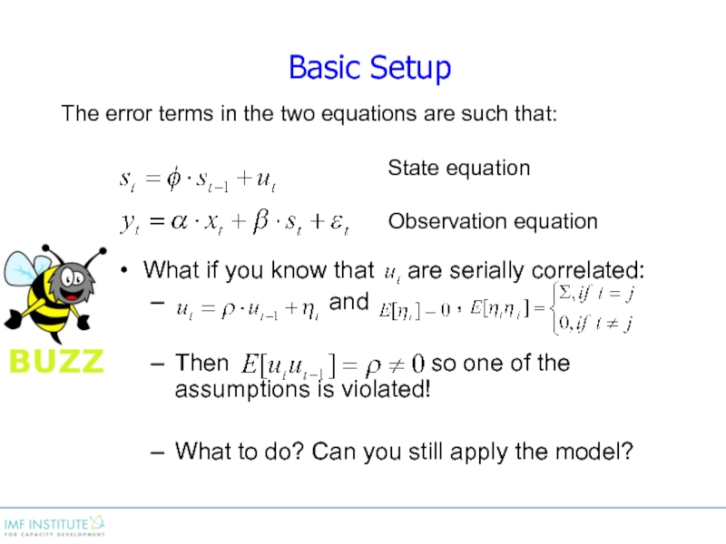
Слайд 16What if you know that are serially correlated:
and ,
Then so one of the assumptions is violated!
What to do? Can you still apply the model?
Basic Setup
The error terms in the two equations are such that:
State equation
Observation equation
Слайд 17The State Space Representation: Examples
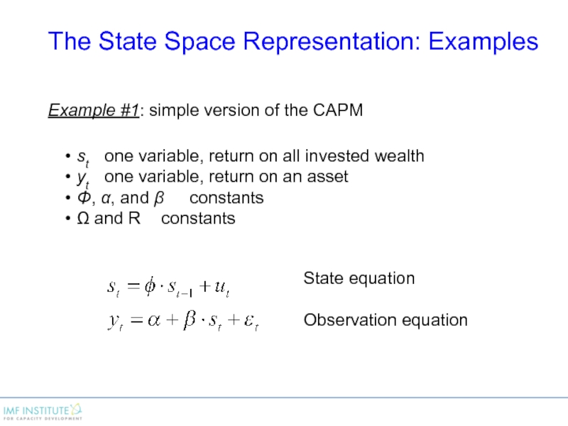
Example #1: simple version of the CAPM
st one
variable, return on all invested wealth
yt one variable, return on an asset
Φ, α, and β constants
Ω and R constants
State equation
Observation equation
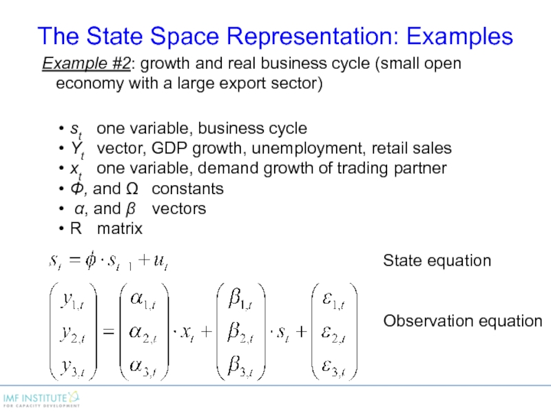
Слайд 18Example #2: growth and real business cycle (small open economy with
a large export sector)
st one variable, business cycle
Yt vector, GDP growth, unemployment, retail sales
xt one variable, demand growth of trading partner
Φ, and Ω constants
α, and β vectors
R matrix
The State Space Representation: Examples
State equation
Observation equation
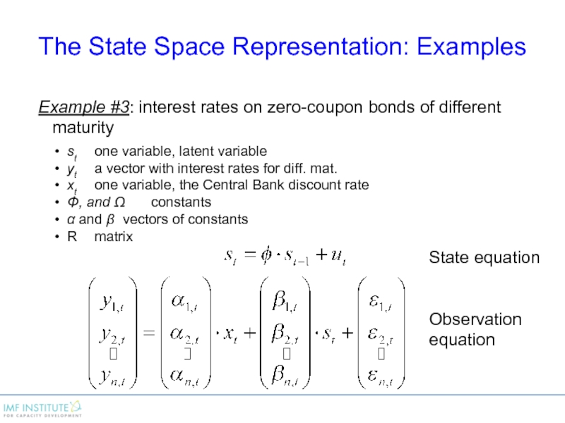
Слайд 19Example #3: interest rates on zero-coupon bonds of different maturity
st one variable,
latent variable
yt a vector with interest rates for diff. mat.
xt one variable, the Central Bank discount rate
Φ, and Ω constants
α and β vectors of constants
R matrix
The State Space Representation: Examples
State equation
Observation equation
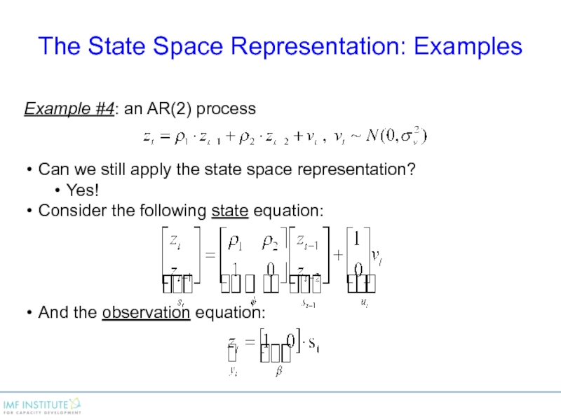
Слайд 20Example #4: an AR(2) process
Can we still apply the state space
representation?
Yes!
Consider the following state equation:
And the observation equation:
The State Space Representation: Examples
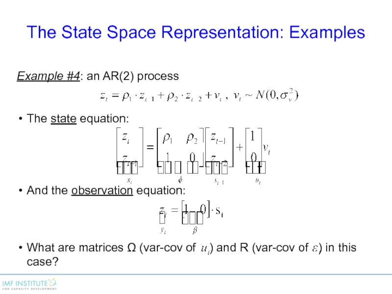
Слайд 21Example #4: an AR(2) process
The state equation:
And the observation equation:
What are
matrices Ω (var-cov of ) and R (var-cov of ) in this case?
The State Space Representation: Examples
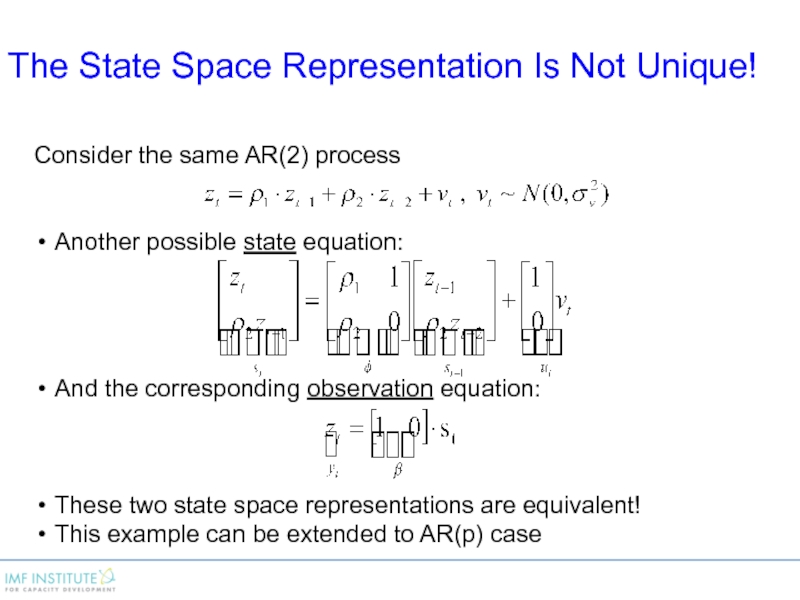
Слайд 22Consider the same AR(2) process
Another possible state equation:
And the corresponding observation
equation:
These two state space representations are equivalent!
This example can be extended to AR(p) case
The State Space Representation Is Not Unique!
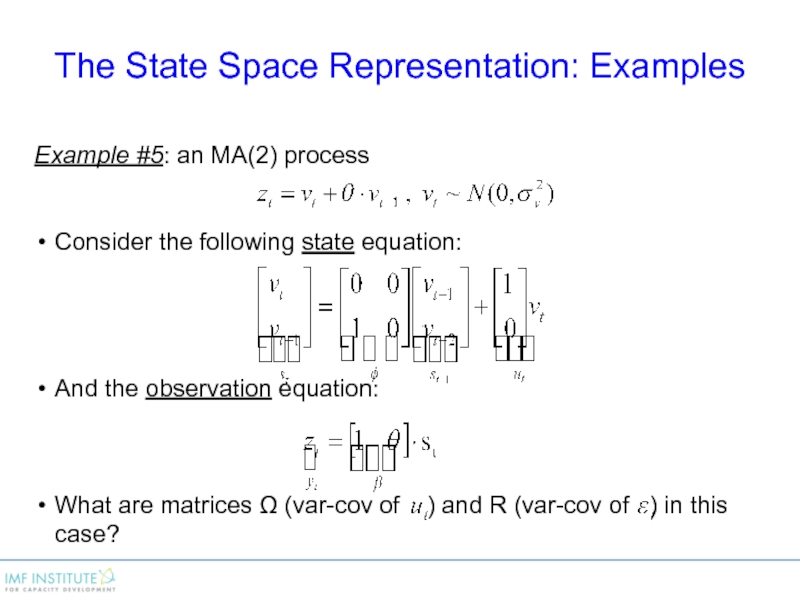
Слайд 23Example #5: an MA(2) process
Consider the following state equation:
And the observation
equation:
What are matrices Ω (var-cov of ) and R (var-cov of ) in this case?
The State Space Representation: Examples
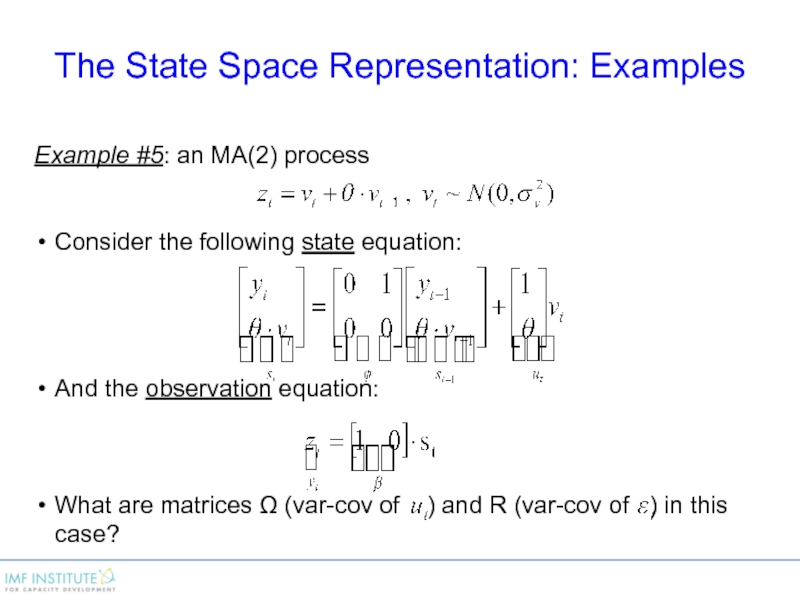
Слайд 24Example #5: an MA(2) process
Consider the following state equation:
And the observation
equation:
What are matrices Ω (var-cov of ) and R (var-cov of ) in this case?
The State Space Representation: Examples
Слайд 25Example #6: A random walk plus drift process
State equation? Observation equation?
What
are the loadings ?
What are matrices Ω (var-cov of ) and R (var-cov of ) for your state-space representation?
The State Space Representation: Examples
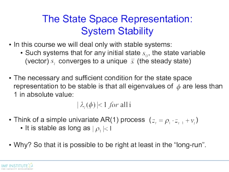
Слайд 26In this course we will deal only with stable systems:
Such systems
that for any initial state , the state variable (vector) converges to a unique (the steady state)
The necessary and sufficient condition for the state space representation to be stable is that all eigenvalues of are less than 1 in absolute value:
Think of a simple univariate AR(1) process ( )
It is stable as long as
Why? So that it is possible to be right at least in the “long-run”.
The State Space Representation:
System Stability
Слайд 28State Space Representation [univariate case]:
Notation:
is the best linear predictor of st conditional on the information up to t-1.
is the best linear predictor of yt conditional on the information up to t-1.
is the best linear predictor of st conditional on the information up to t.
are known
Kalman Filter: Introduction
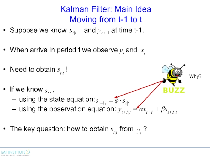
Слайд 29Kalman Filter: Main Idea
Moving from t-1 to t
Suppose we know
and at time t-1.
When arrive in period t we observe and
Need to obtain st|t !
If we know ,
using the state equation:
using the observation equation: yt+1|t = αxt+1 + βst+1|t
The key question: how to obtain st|t from ?
Why?
Слайд 30Kalman Filter: Main Idea
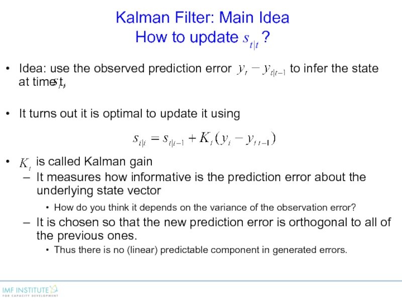
How to update st|t ?
Idea: use the observed
prediction error to infer the state at time t,
It turns out it is optimal to update it using
is called Kalman gain
It measures how informative is the prediction error about the underlying state vector
How do you think it depends on the variance of the observation error?
It is chosen so that the new prediction error is orthogonal to all of the previous ones.
Thus there is no (linear) predictable component in generated errors.
Слайд 31Kalman Filter:
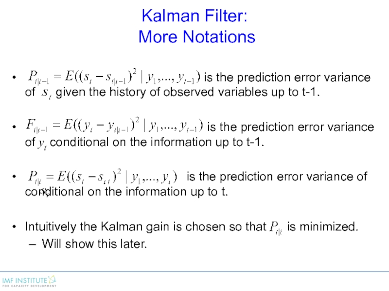
More Notations
is the prediction error variance of given the history of observed variables up to t-1.
is the prediction error variance of yt conditional on the information up to t-1.
is the prediction error variance of conditional on the information up to t.
Intuitively the Kalman gain is chosen so that is minimized.
Will show this later.
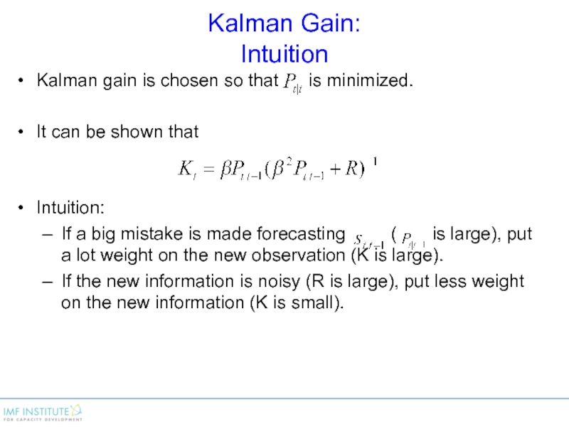
Слайд 32Kalman Gain:
Intuition
Kalman gain is chosen so that is minimized.
It
can be shown that
Intuition:
If a big mistake is made forecasting ( is large), put a lot weight on the new observation (K is large).
If the new information is noisy (R is large), put less weight on the new information (K is small).
Слайд 33Kalman Filter:
Example
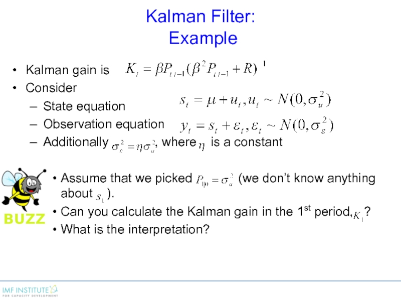
Kalman gain is
Consider
State equation
Observation equation
Additionally
, where is a constant
Assume that we picked (we don’t know anything about ).
Can you calculate the Kalman gain in the 1st period, ?
What is the interpretation?
Слайд 34Kalman Filter:
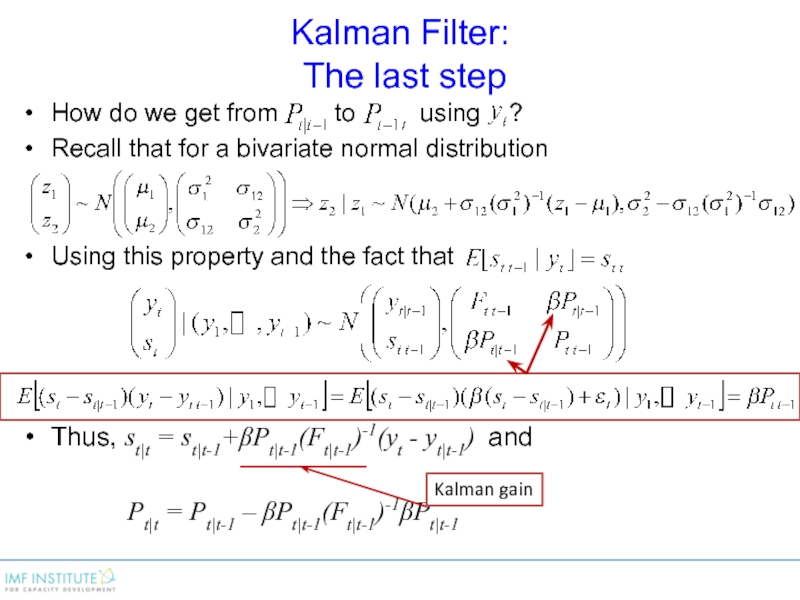
The last step
How do we get from
to using ?
Recall that for a bivariate normal distribution
Using this property and the fact that
Thus, st|t = st|t-1+βPt|t-1(Ft|t-1)-1(yt - yt|t-1) and
Pt|t = Pt|t-1 – βPt|t-1(Ft|t-1)-1βPt|t-1
Kalman gain
Слайд 35Kalman Filter:
Finally
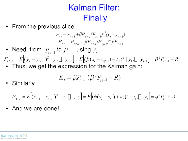
From the previous slide
st|t = st|t-1+βPt|t-1(Ft|t-1)-1(yt - yt|t-1)
Pt|t
= Pt|t-1 – βPt|t-1(Ft|t-1)-1βPt|t-1
Need: from to using
Thus, we get the expression for the Kalman gain:
Similarly
And we are done!
Слайд 36Kalman Filter:
Review
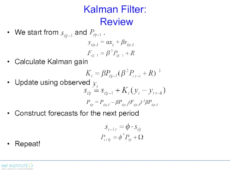
We start from and
.
yt|t-1 = αxt + βst|t-1
Calculate Kalman gain
Update using observed
Construct forecasts for the next period
Repeat!
Pt|t = Pt|t-1 – βPt|t-1(Ft|t-1)-1βPt|t-1
Слайд 37Kalman Filter:
How to choose initial state
If the sample size is
large, the choice of the initial state is not very important
In short samples can have significant effect
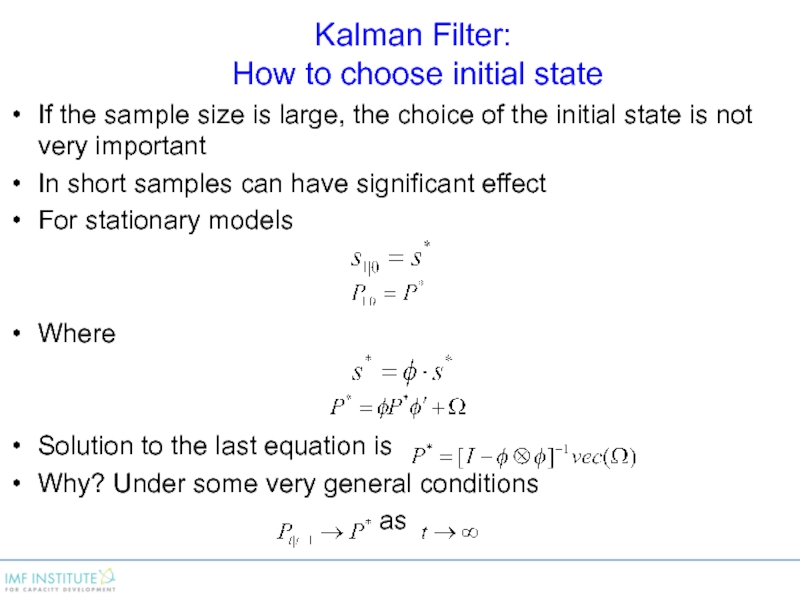
For stationary models
Where
Solution to the last equation is
Why? Under some very general conditions
as
Слайд 38Kalman Filter as a Recursive Regression
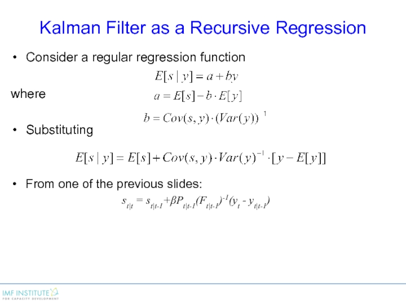
Consider a regular regression function
where
Substituting
From
one of the previous slides:
st|t = st|t-1+βPt|t-1(Ft|t-1)-1(yt - yt|t-1)
Слайд 39Kalman Filter as a Recursive Regression
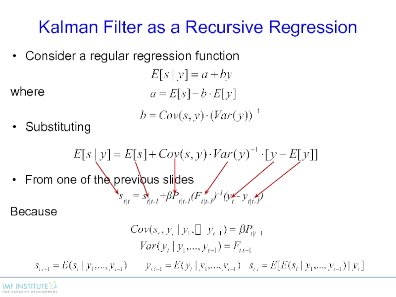
Consider a regular regression function
where
Substituting
From
one of the previous slides
st|t = st|t-1+βPt|t-1(Ft|t-1)-1(yt - yt|t-1)
Because
Слайд 40Kalman Filter as a Recursive Regression
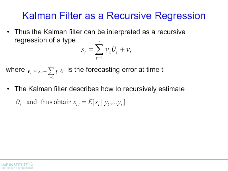
Thus the Kalman filter can be
interpreted as a recursive regression of a type
where is the forecasting error at time t
The Kalman filter describes how to recursively estimate
Слайд 41Optimality of the Kalman Filter
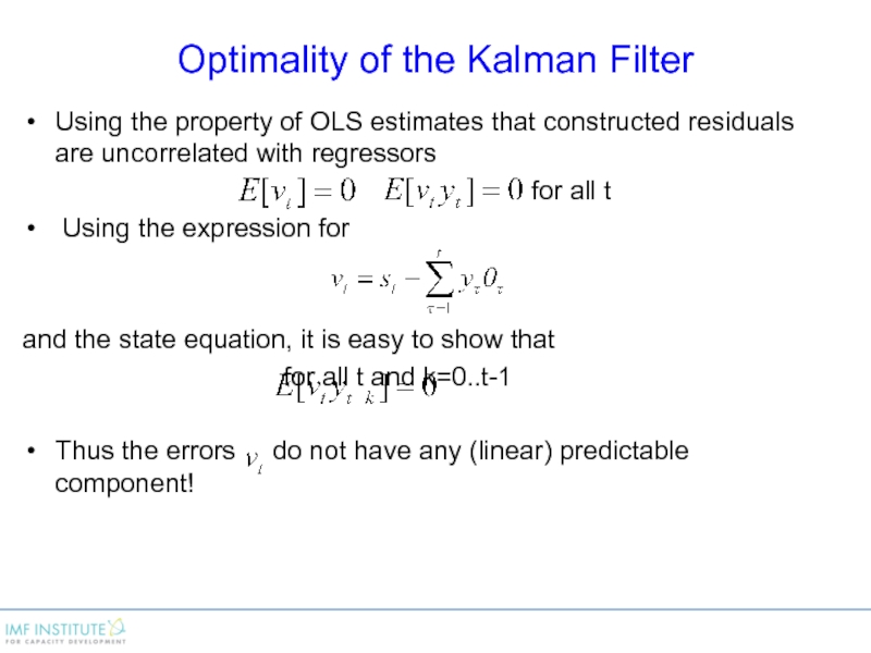
Using the property of OLS estimates that
constructed residuals are uncorrelated with regressors
for all t
Using the expression for
and the state equation, it is easy to show that
for all t and k=0..t-1
Thus the errors do not have any (linear) predictable component!
Слайд 42Kalman Filter
Some comments
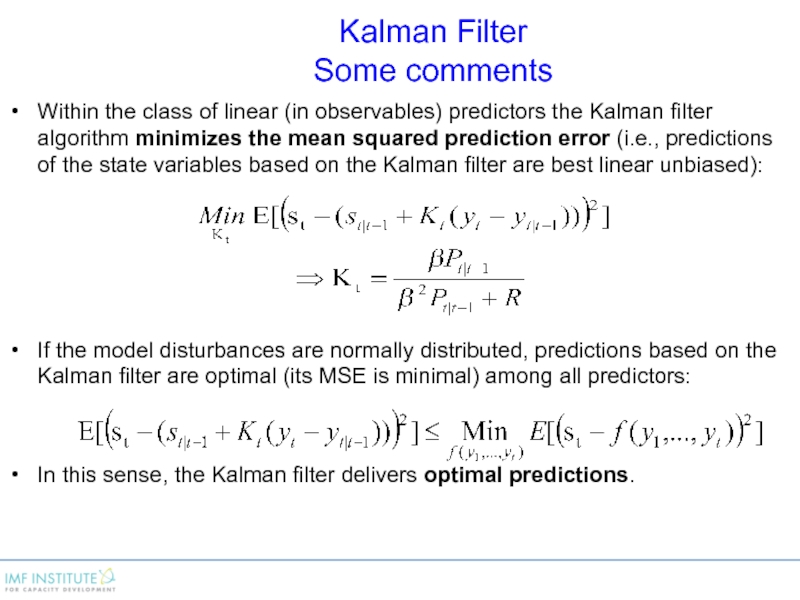
Within the class of linear (in observables) predictors the
Kalman filter algorithm minimizes the mean squared prediction error (i.e., predictions of the state variables based on the Kalman filter are best linear unbiased):
If the model disturbances are normally distributed, predictions based on the Kalman filter are optimal (its MSE is minimal) among all predictors:
In this sense, the Kalman filter delivers optimal predictions.
Слайд 43Kalman Filter - Multivariate Case
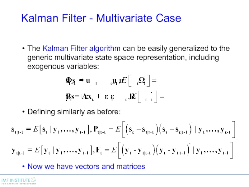
The Kalman Filter algorithm can be easily
generalized to the generic multivariate state space representation, including exogenous variables:
Defining similarly as before:
Now we have vectors and matrices
Слайд 44Kalman Filter Algorithm – Multivariate Case
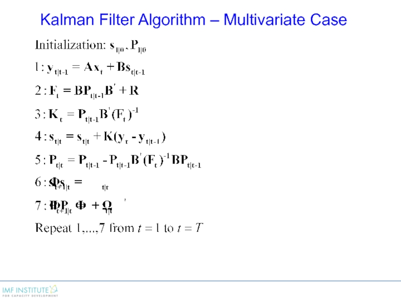
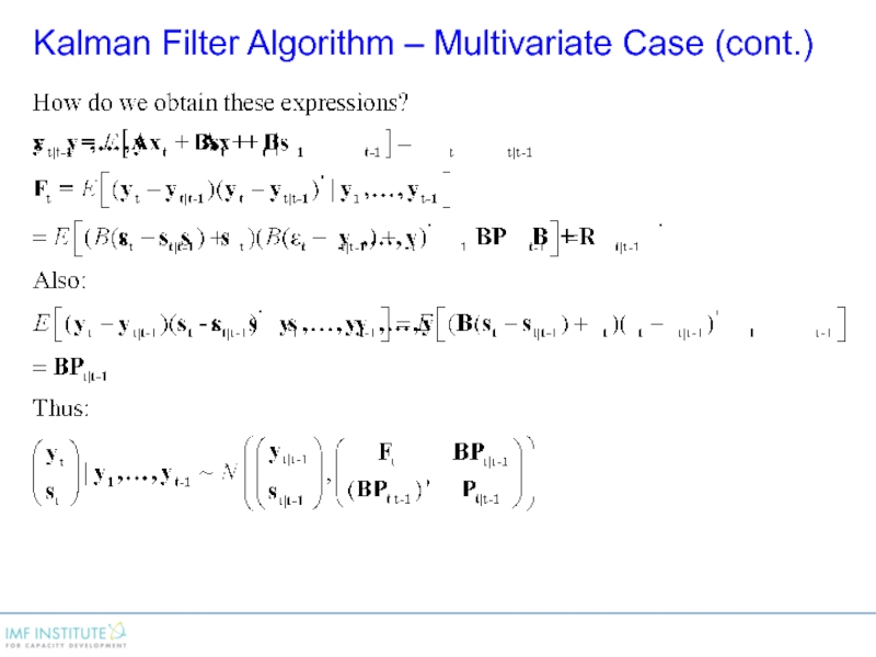
Слайд 45Kalman Filter Algorithm – Multivariate Case (cont.)
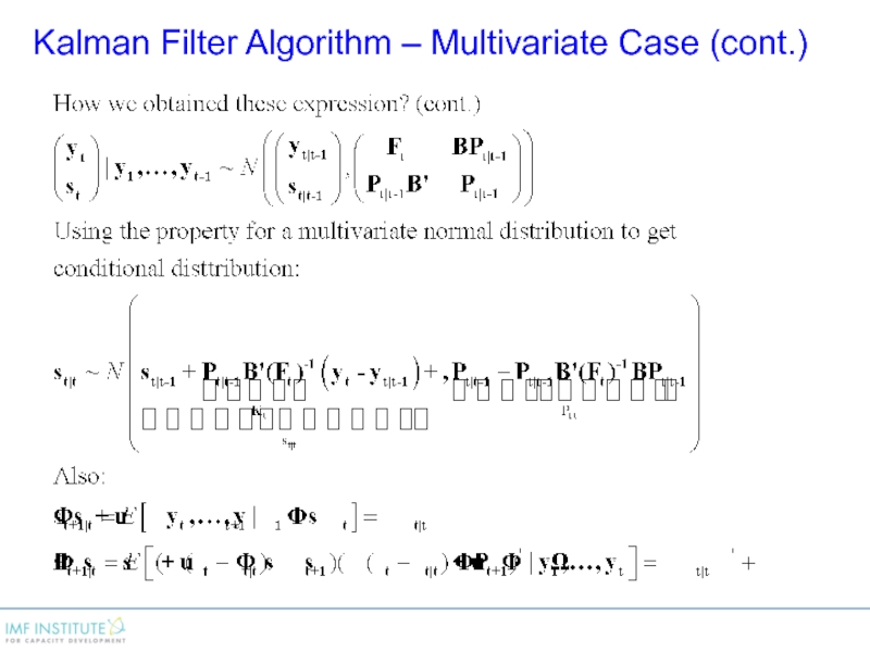
Слайд 46Kalman Filter Algorithm – Multivariate Case (cont.)
Слайд 47ML Estimation and Kalman Smoothing
Слайд 48Maximum Likelihood Estimation
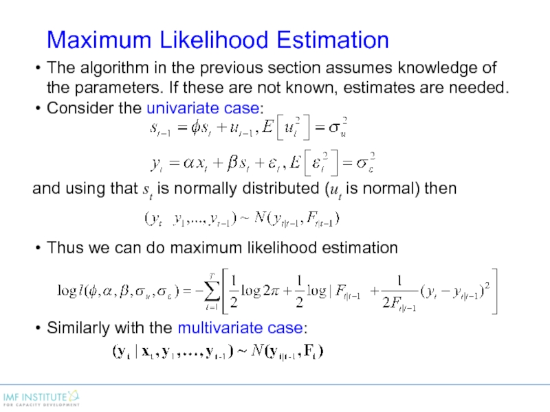
The algorithm in the previous section assumes knowledge of
the parameters. If these are not known, estimates are needed.
Consider the univariate case:
and using that st is normally distributed (ut is normal) then
Thus we can do maximum likelihood estimation
Similarly with the multivariate case:
Слайд 49To estimate model parameters through maximizing log-likelihood:
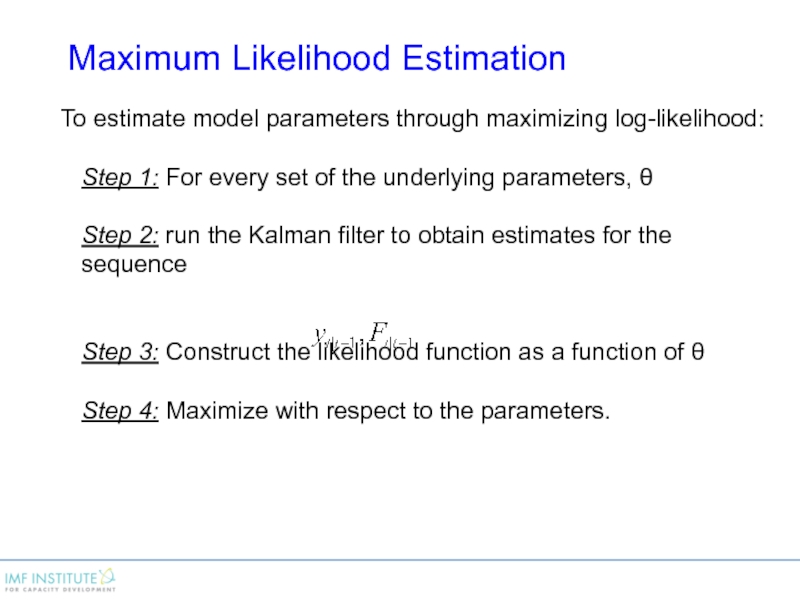
Step 1: For every set
of the underlying parameters, θ
Step 2: run the Kalman filter to obtain estimates for the sequence
Step 3: Construct the likelihood function as a function of θ
Step 4: Maximize with respect to the parameters.
Maximum Likelihood Estimation
Слайд 50Kalman Smoothing
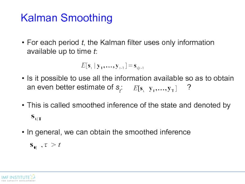
For each period t, the Kalman filter uses only information
available up to time t:
Is it possible to use all the information available so as to obtain an even better estimate of st: ?
This is called smoothed inference of the state and denoted by
In general, we can obtain the smoothed inference
Слайд 51Kalman Smoothing
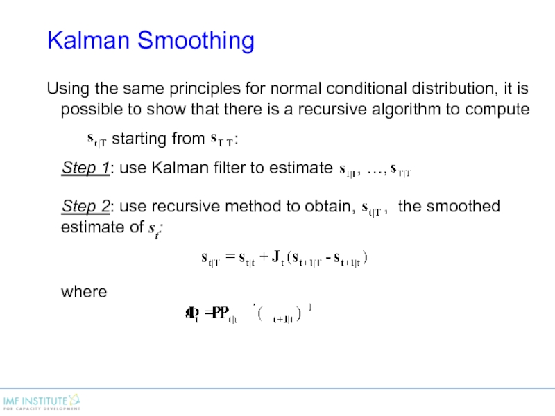
Using the same principles for normal conditional distribution, it is
possible to show that there is a recursive algorithm to compute
starting from :
Step 1: use Kalman filter to estimate , …,
Step 2: use recursive method to obtain, , the smoothed estimate of st:
where
Слайд 52Conclusion
Many models require estimations of unobserved variables, either because these are
of economic interest, or because one needs them to estimate the model parameters (example, ARMA).
The Kalman filter is a recursive algorithm that:
provides efficient estimates of unobserved variables, and their MSE;
can be used for forecasting given estimates of MSE;
is used to initialize maximum likelihood estimation of models (for example, of ARMA models) by first producing good estimates of un-observed variables;
can also be used to smooth series for unobserved variables.



![State Space Representation [univariate case]:Notation: is](/img/tmb/4/358739/83856d7dff99239cbe1efbba66f78b41-800x.jpg)
