- Главная
- Разное
- Дизайн
- Бизнес и предпринимательство
- Аналитика
- Образование
- Развлечения
- Красота и здоровье
- Финансы
- Государство
- Путешествия
- Спорт
- Недвижимость
- Армия
- Графика
- Культурология
- Еда и кулинария
- Лингвистика
- Английский язык
- Астрономия
- Алгебра
- Биология
- География
- Детские презентации
- Информатика
- История
- Литература
- Маркетинг
- Математика
- Медицина
- Менеджмент
- Музыка
- МХК
- Немецкий язык
- ОБЖ
- Обществознание
- Окружающий мир
- Педагогика
- Русский язык
- Технология
- Физика
- Философия
- Химия
- Шаблоны, картинки для презентаций
- Экология
- Экономика
- Юриспруденция
Cost-Volume-Profit (CVP) Analysis презентация
Содержание
- 1. Cost-Volume-Profit (CVP) Analysis
- 2. Basic Assumptions Changes in production/sales volume are
- 3. Basic Assumptions, continued Selling price, variable cost
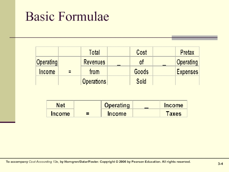
- 4. Basic Formulae
- 5. Contribution Margin Contribution Margin equals sales less
- 6. Contribution Margin Contribution Margin also equals contribution
- 7. Contribution Margin Income Statement Derivations A
- 8. CVP, Graphically Total costs line Operating loss
- 9. Breakeven Point Recall the last equation in
- 10. Breakeven Point, continued If per-unit values are
- 11. Breakeven Point, extended: Profit Planning With
- 12. CVP and Income Taxes From time to
- 13. Sensitivity Analysis CVP provides structure to answer
- 14. Margin of Safety One indicator of risk,
- 15. Operating Leverage Operating Leverage (OL) is the
- 16. Effects of Sales-Mix on CVP The formulae
- 17. Effects of Sales-Mix on CVP A weighted-average
- 18. Multiple Cost Drivers Variable costs may arise
- 19. Contribution Margin vs. Gross Profit Comparative Statements
Слайд 2Basic Assumptions
Changes in production/sales volume are the sole cause for cost
and revenue changes
Total costs consist of fixed costs and variable costs
Revenue and costs behave and can be graphed as a linear function (a straight line)
Total costs consist of fixed costs and variable costs
Revenue and costs behave and can be graphed as a linear function (a straight line)
Слайд 3Basic Assumptions, continued
Selling price, variable cost per unit, and fixed costs
are all known and constant
In many cases only a single product will be analyzed. If multiple products are studied, their relative sales proportions are known and constant
The time value of money (interest) is ignored
In many cases only a single product will be analyzed. If multiple products are studied, their relative sales proportions are known and constant
The time value of money (interest) is ignored
Слайд 5Contribution Margin
Contribution Margin equals sales less variable costs
CM = S
– VC
Contribution Margin per unit equals unit selling price less variable cost per unit
CMu = SP – VCu
Contribution Margin per unit equals unit selling price less variable cost per unit
CMu = SP – VCu
Слайд 6Contribution Margin
Contribution Margin also equals contribution margin per unit multiplied by
the number of units sold
CM = CMu x Q
Contribution Margin Ratio (percentage) equals contribution margin per unit divided by selling price
CMR = CMu ÷ SP
CM = CMu x Q
Contribution Margin Ratio (percentage) equals contribution margin per unit divided by selling price
CMR = CMu ÷ SP
Слайд 7Contribution Margin
Income Statement Derivations
A horizontal presentation of the Contribution Margin
Income Statement:
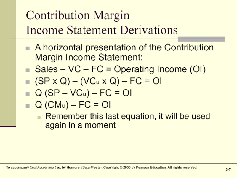
Sales – VC – FC = Operating Income (OI)
(SP x Q) – (VCu x Q) – FC = OI
Q (SP – VCu) – FC = OI
Q (CMu) – FC = OI
Remember this last equation, it will be used again in a moment
Sales – VC – FC = Operating Income (OI)
(SP x Q) – (VCu x Q) – FC = OI
Q (SP – VCu) – FC = OI
Q (CMu) – FC = OI
Remember this last equation, it will be used again in a moment
Слайд 8CVP, Graphically
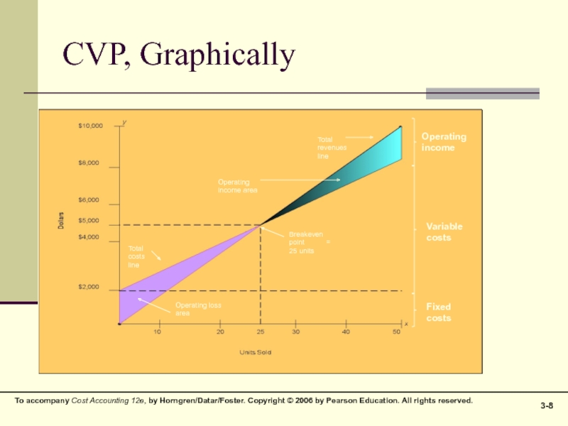
Total costs line
Operating loss area
Breakeven point = 25 units
Total costs
line
Operating loss area
Operating income area
Breakeven point = 25 units
Total revenues line
Operating income
Variable costs
Fixed costs
Слайд 9Breakeven Point
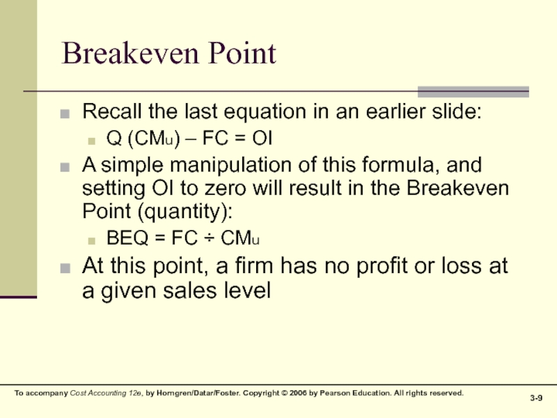
Recall the last equation in an earlier slide:
Q (CMu) –
FC = OI
A simple manipulation of this formula, and setting OI to zero will result in the Breakeven Point (quantity):
BEQ = FC ÷ CMu
At this point, a firm has no profit or loss at a given sales level
A simple manipulation of this formula, and setting OI to zero will result in the Breakeven Point (quantity):
BEQ = FC ÷ CMu
At this point, a firm has no profit or loss at a given sales level
Слайд 10Breakeven Point, continued
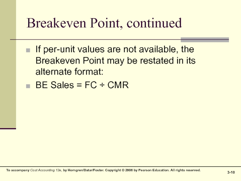
If per-unit values are not available, the Breakeven Point
may be restated in its alternate format:
BE Sales = FC ÷ CMR
BE Sales = FC ÷ CMR
Слайд 11Breakeven Point, extended:
Profit Planning
With a simple adjustment, the Breakeven Point
formula can be modified to become a Profit Planning tool
Profit is now reinstated to the BE formula, changing it to a simple sales volume equation
Q = (FC + OI)
CM
Profit is now reinstated to the BE formula, changing it to a simple sales volume equation
Q = (FC + OI)
CM
Слайд 12CVP and Income Taxes
From time to time it is necessary to
move back and forth between pre-tax profit (OI) and after-tax profit (NI), depending on the facts presented
After-tax profit can be calculated by:
OI x (1-Tax Rate) = NI
NI can substitute into the profit planning equation through this form:
OI = I I NI I
(1-Tax Rate)
After-tax profit can be calculated by:
OI x (1-Tax Rate) = NI
NI can substitute into the profit planning equation through this form:
OI = I I NI I
(1-Tax Rate)
Слайд 13Sensitivity Analysis
CVP provides structure to answer a variety of “what-if” scenarios
“What”
happens to profit “if”:
Selling price changes
Volume changes
Cost structure changes
Variable cost per unit changes
Fixed cost changes
Selling price changes
Volume changes
Cost structure changes
Variable cost per unit changes
Fixed cost changes
Слайд 14Margin of Safety
One indicator of risk, the Margin of Safety (MOS)
measures the distance between budgeted sales and breakeven sales:
MOS = Budgeted Sales – BE Sales
The MOS Ratio removes the firm’s size from the output, and expresses itself in the form of a percentage:
MOS Ratio = MOS ÷ Budgeted Sales
MOS = Budgeted Sales – BE Sales
The MOS Ratio removes the firm’s size from the output, and expresses itself in the form of a percentage:
MOS Ratio = MOS ÷ Budgeted Sales
Слайд 15Operating Leverage
Operating Leverage (OL) is the effect that fixed costs have
on changes in operating income as changes occur in units sold, expressed as changes in contribution margin
OL = Contribution Margin
Operating Income
Notice these two items are identical, except for fixed costs
OL = Contribution Margin
Operating Income
Notice these two items are identical, except for fixed costs
Слайд 16Effects of Sales-Mix on CVP
The formulae presented to this point have
assumed a single product is produced and sold
A more realistic scenario involves multiple products sold, in different volumes, with different costs
For simplicity’s sake, only two products will be presented, but this could easily be extended to even more products
A more realistic scenario involves multiple products sold, in different volumes, with different costs
For simplicity’s sake, only two products will be presented, but this could easily be extended to even more products
Слайд 17Effects of Sales-Mix on CVP
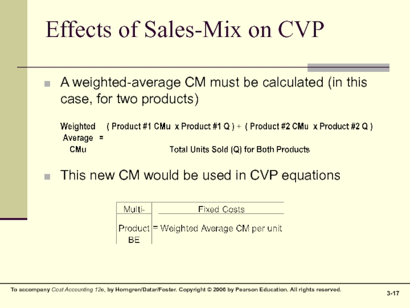
A weighted-average CM must be calculated (in
this case, for two products)
This new CM would be used in CVP equations
This new CM would be used in CVP equations
Слайд 18Multiple Cost Drivers
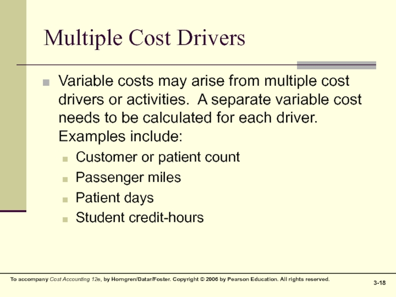
Variable costs may arise from multiple cost drivers or
activities. A separate variable cost needs to be calculated for each driver. Examples include:
Customer or patient count
Passenger miles
Patient days
Student credit-hours
Customer or patient count
Passenger miles
Patient days
Student credit-hours
