- Главная
- Разное
- Дизайн
- Бизнес и предпринимательство
- Аналитика
- Образование
- Развлечения
- Красота и здоровье
- Финансы
- Государство
- Путешествия
- Спорт
- Недвижимость
- Армия
- Графика
- Культурология
- Еда и кулинария
- Лингвистика
- Английский язык
- Астрономия
- Алгебра
- Биология
- География
- Детские презентации
- Информатика
- История
- Литература
- Маркетинг
- Математика
- Медицина
- Менеджмент
- Музыка
- МХК
- Немецкий язык
- ОБЖ
- Обществознание
- Окружающий мир
- Педагогика
- Русский язык
- Технология
- Физика
- Философия
- Химия
- Шаблоны, картинки для презентаций
- Экология
- Экономика
- Юриспруденция
Depressions and Slumps презентация
Содержание
- 1. Depressions and Slumps
- 2. 22-1 Disinflation, Deflation, and the Liquidity Trap
- 3. Recall from Chapter 7 and this graph
- 4. Chapters 8 and 9 presented a more
- 5. The built-in mechanism that can lift economies
- 6. Recall from Chapter 14 that: What
- 7. 22-1 Disinflation, Deflation, and the Liquidity Trap
- 8. Because output is below the natural level
- 9. 22-1 Disinflation, Deflation, and the Liquidity Trap
- 10. The demand for money is as shown
- 11. Now consider the effects of an increase
- 12. The liquidity trap describes a situation in
- 13. 22-1 Disinflation, Deflation, and the Liquidity Trap
- 14. 22-1 Disinflation, Deflation, and the Liquidity Trap
- 15. 22-1 Disinflation, Deflation, and the Liquidity Trap
- 16. 22-1 Disinflation, Deflation, and the Liquidity Trap
- 17. At a negative real interest rate of
- 18. 22-1 Disinflation, Deflation, and the Liquidity Trap
- 19. 22-2 The Great Depression The Great Depression
- 20. 22-2 The Great Depression
- 21. Focusing only on unemployment and output for
- 22. The Initial Fall in Spending 22-2 The
- 23. The Contraction in Nominal Money 22-2 The
- 24. The Contraction in Nominal Money 22-2 The
- 25. The result of low output was strong
- 26. Monetary policy played an important role in
- 27. The puzzle is why deflation ended in
- 28. The robust growth that Japan had experienced
- 29. 22-3 The Japanese Slump From 1992 to
- 30. 22-3 The Japanese Slump Low growth in
- 31. 22-3 The Japanese Slump The numbers in
- 32. There are two reasons for the increase
- 33. 22-3 The Japanese Slump The Rise and
- 34. The fact that dividends remained flat while
- 35. 22-3 The Japanese Slump The Failure of
- 36. Monetary policy was used, but it was
- 37. Fiscal policy was used as well. Taxes
- 38. 22-3 The Japanese Slump The Failure of
- 39. Output growth has been higher since 2003,
- 40. It is suggested that even if the
- 41. The Japanese Banking Problem Like
- 42. Key Terms depression slump liquidity trap New
Слайд 1Depressions and Slumps
A depression is a deep and long-lasting recession.
A slump
Слайд 222-1 Disinflation, Deflation,
and the Liquidity Trap
Low output leads to a decrease
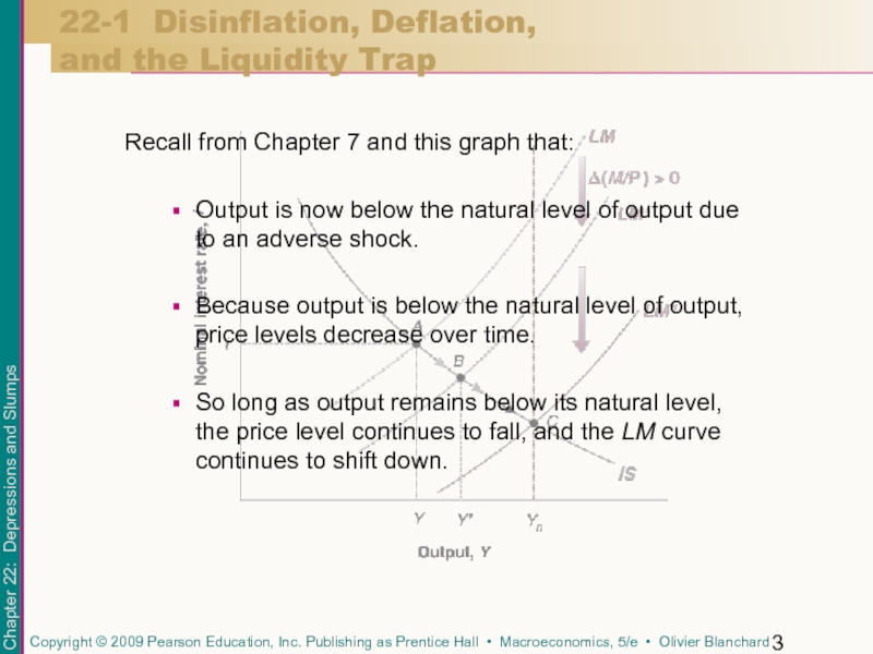
Слайд 3Recall from Chapter 7 and this graph that:
Output is now below
Because output is below the natural level of output, price levels decrease over time.
So long as output remains below its natural level, the price level continues to fall, and the LM curve continues to shift down.
22-1 Disinflation, Deflation,
and the Liquidity Trap
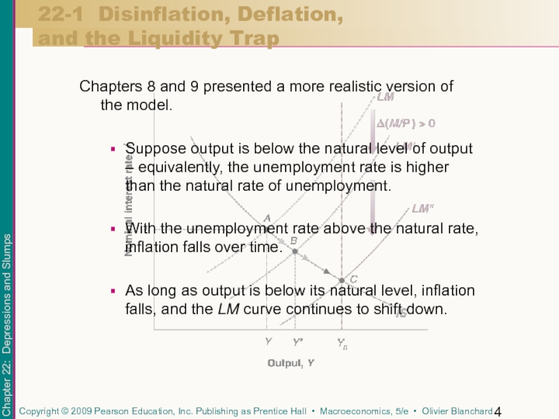
Слайд 4Chapters 8 and 9 presented a more realistic version of the
Suppose output is below the natural level of output – equivalently, the unemployment rate is higher than the natural rate of unemployment.
With the unemployment rate above the natural rate, inflation falls over time.
As long as output is below its natural level, inflation falls, and the LM curve continues to shift down.
22-1 Disinflation, Deflation,
and the Liquidity Trap
Слайд 5The built-in mechanism that can lift economies out of recessions is
Output below the natural level of output leads to lower inflation.
Lower inflation leads in turn to higher real money growth.
Higher real money growth leads to an increase in output over time.
This mechanism, however, is not foolproof.
22-1 Disinflation, Deflation,
and the Liquidity Trap
Слайд 6Recall from Chapter 14 that:
What matters for spending decisions, and thus
What matters for the demand for money, and thus enters the LM relation, is the nominal interest rate—the interest rate in terms of dollars.
22-1 Disinflation, Deflation,
and the Liquidity Trap
The Nominal Interest Rate, the Real Interest Rate,
and Expected Inflation
Слайд 722-1 Disinflation, Deflation,
and the Liquidity Trap
The Nominal Interest Rate, the Real
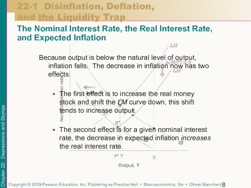
When inflation decreases in response to low output, there are two effects: (1) The real money stock increases, leading the LM curve to shift down, and (2) expected inflation decreases, leading the IS curve to shift to the left. The result may be a further decrease in output.
Слайд 8Because output is below the natural level of output, inflation falls.
The first effect is to increase the real money stock and shift the LM curve down, this shift tends to increase output.
The second effect is for a given nominal interest rate, the decrease in expected inflation increases the real interest rate.
22-1 Disinflation, Deflation,
and the Liquidity Trap
The Nominal Interest Rate, the Real Interest Rate,
and Expected Inflation
Слайд 922-1 Disinflation, Deflation,
and the Liquidity Trap
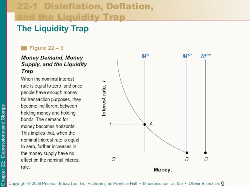
The Liquidity Trap
When the nominal interest
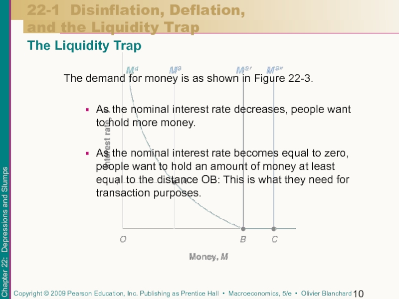
Слайд 10The demand for money is as shown in Figure 22-3.
As the
As the nominal interest rate becomes equal to zero, people want to hold an amount of money at least equal to the distance OB: This is what they need for transaction purposes.
22-1 Disinflation, Deflation,
and the Liquidity Trap
The Liquidity Trap
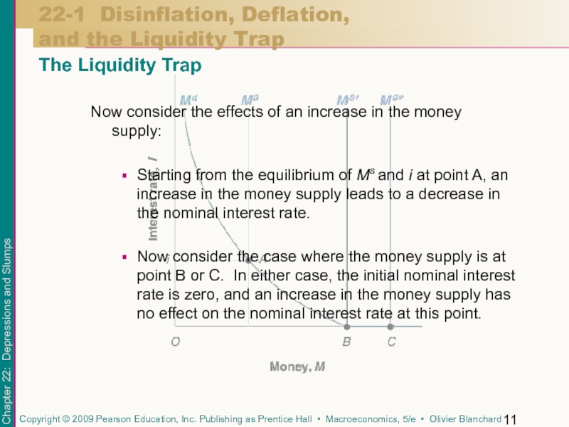
Слайд 11Now consider the effects of an increase in the money supply:
Starting
Now consider the case where the money supply is at point B or C. In either case, the initial nominal interest rate is zero, and an increase in the money supply has no effect on the nominal interest rate at this point.
22-1 Disinflation, Deflation,
and the Liquidity Trap
The Liquidity Trap
Слайд 12The liquidity trap describes a situation in which expansionary monetary policy
The central bank can increase “liquidity” but the additional money is willingly held by financial investors at an unchanged interest rate, namely, zero.
22-1 Disinflation, Deflation,
and the Liquidity Trap
The Liquidity Trap
Слайд 1322-1 Disinflation, Deflation,
and the Liquidity Trap
The Liquidity Trap
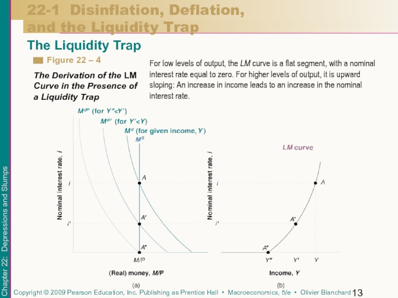
For low levels of
Слайд 1422-1 Disinflation, Deflation,
and the Liquidity Trap
The Liquidity Trap
To derive the LM
The combination of income, Y, and nominal interest rate, i, gives us the first point on the LM curve, point A in Figure 22-4(b).
Lower income means fewer transactions, and, therefore, a lower demand for money at any interest rate. This combination of income, Y’, and nominal interest rate, i’, gives us the second point on the LM curve, point A’ in Figure 22-4(b).
Слайд 1522-1 Disinflation, Deflation,
and the Liquidity Trap
The Liquidity Trap
The equilibrium is given
The intersection between the money supply curve and the money demand curve takes place on the horizontal portion of the money demand curve. The equilibrium remains at A”, and the nominal interest rate remains equal to zero.
Слайд 1622-1 Disinflation, Deflation,
and the Liquidity Trap
The Liquidity Trap
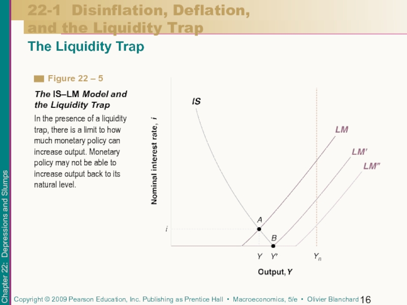
In the presence of
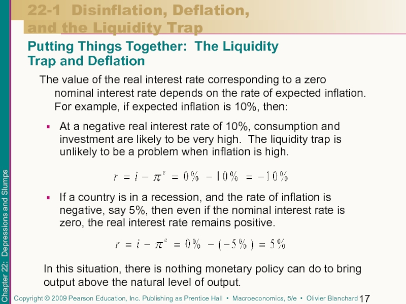
Слайд 17At a negative real interest rate of 10%, consumption and investment
If a country is in a recession, and the rate of inflation is negative, say 5%, then even if the nominal interest rate is zero, the real interest rate remains positive.
The value of the real interest rate corresponding to a zero nominal interest rate depends on the rate of expected inflation. For example, if expected inflation is 10%, then:
22-1 Disinflation, Deflation,
and the Liquidity Trap
Putting Things Together: The Liquidity
Trap and Deflation
In this situation, there is nothing monetary policy can do to bring output above the natural level of output.
Слайд 1822-1 Disinflation, Deflation,
and the Liquidity Trap
Putting Things Together: The Liquidity
Trap
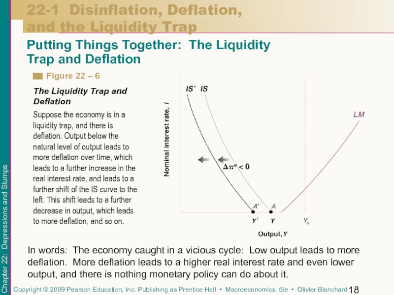
In words: The economy caught in a vicious cycle: Low output leads to more deflation. More deflation leads to a higher real interest rate and even lower output, and there is nothing monetary policy can do about it.
Suppose the economy is in a liquidity trap, and there is deflation. Output below the natural level of output leads to more deflation over time, which leads to a further increase in the real interest rate, and leads to a further shift of the IS curve to the left. This shift leads to a further decrease in output, which leads to more deflation, and so on.
Слайд 1922-2 The Great Depression
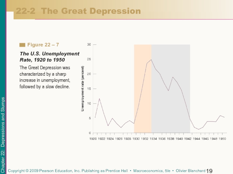
The Great Depression was characterized by a sharp
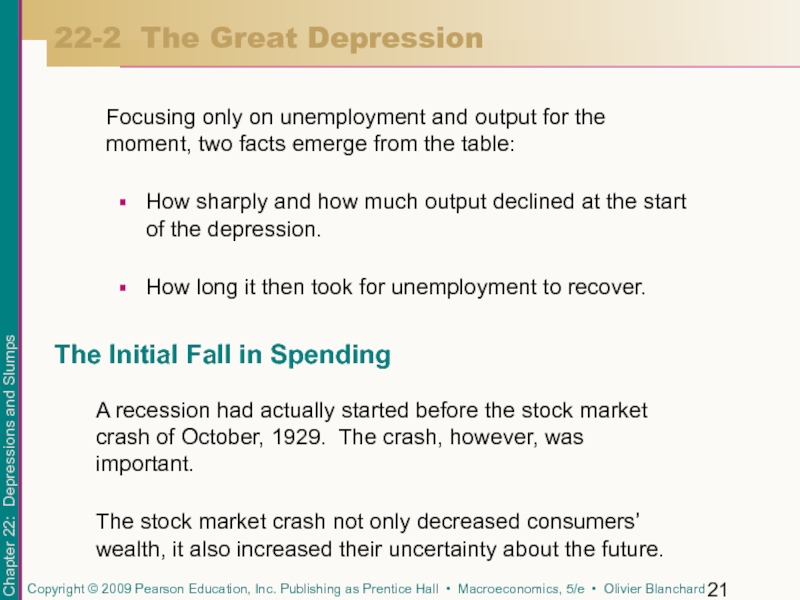
Слайд 21Focusing only on unemployment and output for the moment, two facts
How sharply and how much output declined at the start of the depression.
How long it then took for unemployment to recover.
22-2 The Great Depression
A recession had actually started before the stock market crash of October, 1929. The crash, however, was important.
The stock market crash not only decreased consumers’ wealth, it also increased their uncertainty about the future.
The Initial Fall in Spending
Слайд 22The Initial Fall in Spending
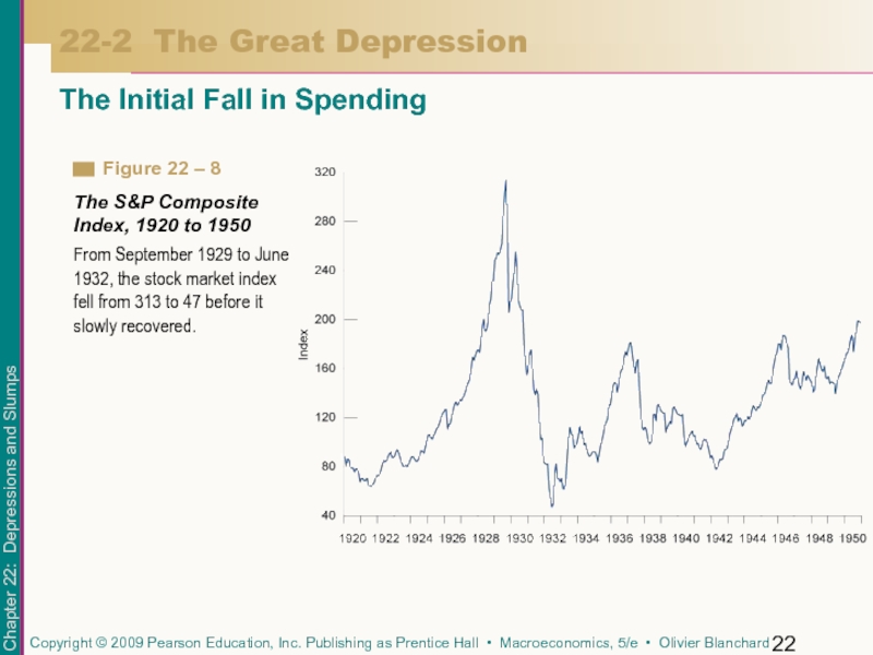
22-2 The Great Depression
From September 1929 to
Слайд 23The Contraction in Nominal Money
22-2 The Great Depression
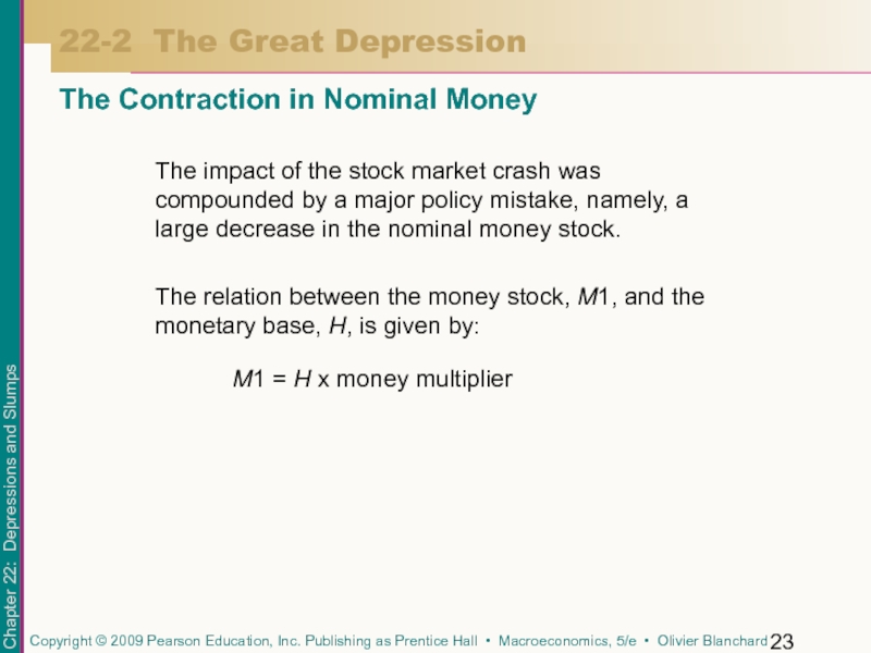
The impact of the
The relation between the money stock, M1, and the monetary base, H, is given by:
M1 = H x money multiplier
Слайд 24The Contraction in Nominal Money
22-2 The Great Depression
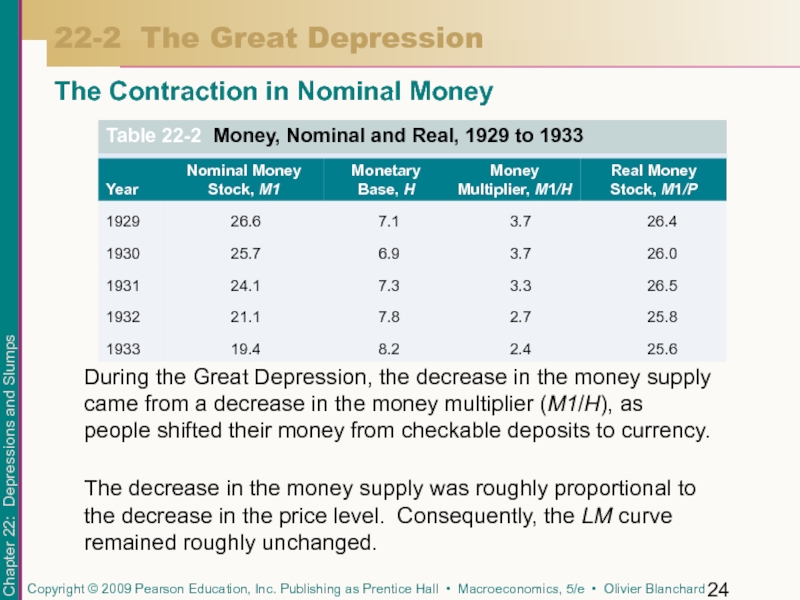
During the Great Depression,
The decrease in the money supply was roughly proportional to the decrease in the price level. Consequently, the LM curve remained roughly unchanged.
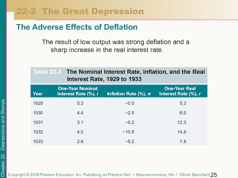
Слайд 25The result of low output was strong deflation and a sharp
The Adverse Effects of Deflation
22-2 The Great Depression
Слайд 26Monetary policy played an important role in the recovery. From 1933
The Recovery
22-2 The Great Depression
Other factors that played an important role were:
The New Deal—a set of programs implemented by the Roosevelt administration.
The creation of the Federal Deposit Insurance Corporation (FDIC).
Other programs administered by the National Recovery Administration (NRA).
Слайд 27The puzzle is why deflation ended in 1933.
One proximate cause may
Another factor may be that while unemployment was still high, output growth was high as well.
Another factor may be the perception of a “regime change” associated with the election of Roosevelt.
The Recovery
22-2 The Great Depression
Слайд 28The robust growth that Japan had experienced since the end of
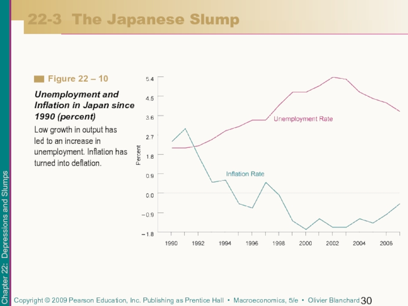
Since 1992, the economy has suffered from a long period of low growth—what is called the Japanese slump.
Low growth has led to a steady increase in unemployment, and a steady decrease in the inflation rate over time.
22-3 The Japanese Slump
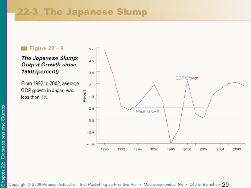
Слайд 3022-3 The Japanese Slump
Low growth in output has led to an
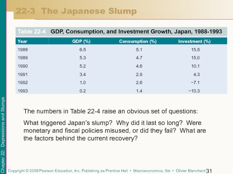
Слайд 3122-3 The Japanese Slump
The numbers in Table 22-4 raise an obvious
What triggered Japan’s slump? Why did it last so long? Were monetary and fiscal policies misused, or did they fail? What are the factors behind the current recovery?
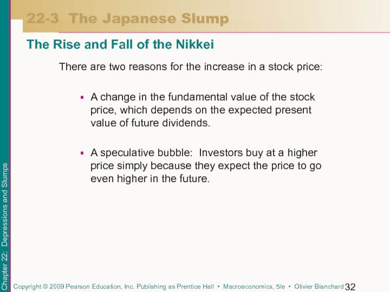
Слайд 32There are two reasons for the increase in a stock price:
A
A speculative bubble: Investors buy at a higher price simply because they expect the price to go even higher in the future.
22-3 The Japanese Slump
The Rise and Fall of the Nikkei
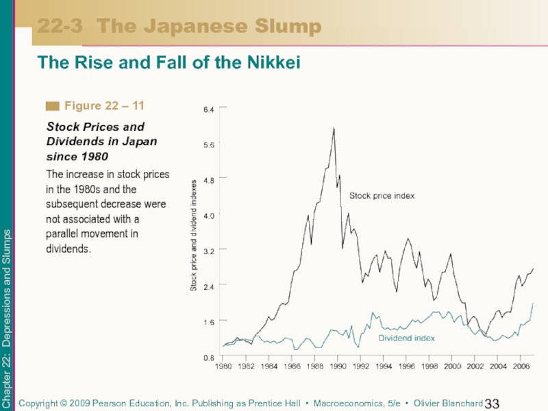
Слайд 3322-3 The Japanese Slump
The Rise and Fall of the Nikkei
The increase
Слайд 34The fact that dividends remained flat while stock prices increased strongly
The rapid fall in stock prices had a major impact on spending—consumption was less affected, but investment collapsed.
22-3 The Japanese Slump
The Rise and Fall of the Nikkei
Слайд 3522-3 The Japanese Slump
The Failure of Monetary and Fiscal Policy
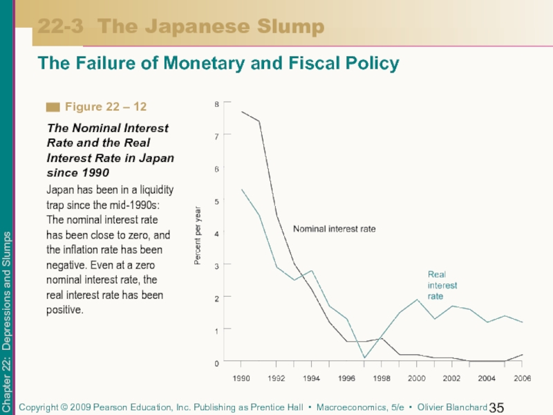
Japan has
Слайд 36Monetary policy was used, but it was used too late, and
The Bank of Japan (BoJ) cut the nominal interest rate, but it did so slowly, and the cumulative effect of low growth was such that inflation had turned to deflation. As a result, the real interest rate was higher than the nominal interest rate.
22-3 The Japanese Slump
The Failure of Monetary and Fiscal Policy
Слайд 37Fiscal policy was used as well. Taxes decreased at the start
Fiscal policy helped, but it was not enough to increase spending and output.
22-3 The Japanese Slump
The Failure of Monetary and Fiscal Policy
Слайд 3822-3 The Japanese Slump
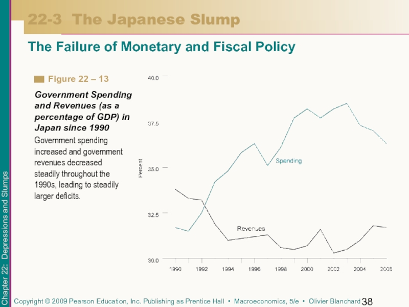
The Failure of Monetary and Fiscal Policy
Government spending
Слайд 39Output growth has been higher since 2003, and most economists cautiously
There appear to be two main factors.
22-3 The Japanese Slump
The Japanese Recovery
Слайд 40It is suggested that even if the nominal interest rate is
22-3 The Japanese Slump
The Japanese Recovery
A Regime Change in Monetary Policy
It became clear in the 1990s that the banking system in Japan was in trouble. Since 2002, the government has put increasing pressure on banks to reduce bad loans, and banks, in turn, have put increasing pressure on bad firms to restructure or close.
The Cleanup of the Banking System
Слайд 41
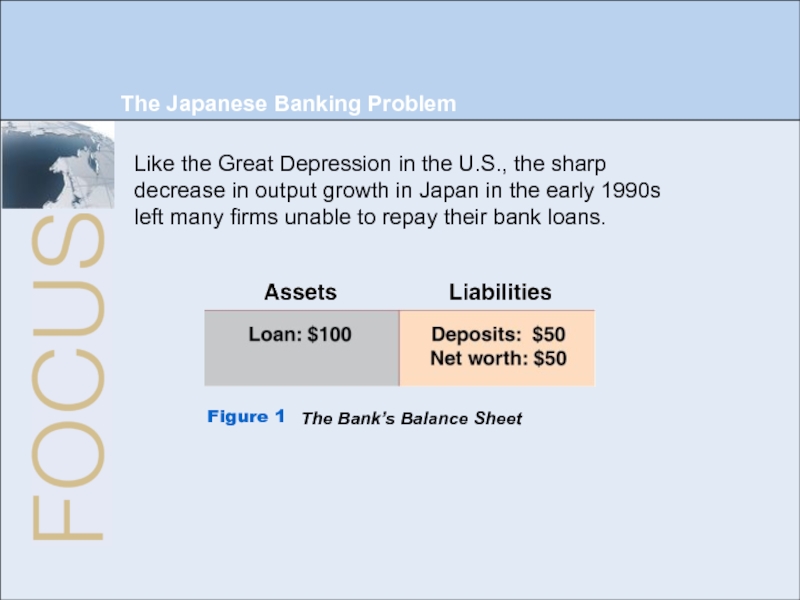
The Japanese Banking Problem
Like the Great Depression in the U.S., the
Figure 1
The Bank’s Balance Sheet


