- Главная
- Разное
- Дизайн
- Бизнес и предпринимательство
- Аналитика
- Образование
- Развлечения
- Красота и здоровье
- Финансы
- Государство
- Путешествия
- Спорт
- Недвижимость
- Армия
- Графика
- Культурология
- Еда и кулинария
- Лингвистика
- Английский язык
- Астрономия
- Алгебра
- Биология
- География
- Детские презентации
- Информатика
- История
- Литература
- Маркетинг
- Математика
- Медицина
- Менеджмент
- Музыка
- МХК
- Немецкий язык
- ОБЖ
- Обществознание
- Окружающий мир
- Педагогика
- Русский язык
- Технология
- Физика
- Философия
- Химия
- Шаблоны, картинки для презентаций
- Экология
- Экономика
- Юриспруденция
Aggregated supply and demand презентация
Содержание
- 1. Aggregated supply and demand
- 2. Aggregate Demand (AD) Aggregate demand is the
- 3. AD shifts AD = C+I+G+NX change in
- 4. Components of AS Consumer goods. Private consumer goods
- 5. Long-run Aggregate supply (LRAS) Supply = capability
- 6. Sort-run Aggregate Supply (SRAS) Rising the price
- 7. Summirising Aggregate supply is the total quantity of
- 8. Equilibrium in the aggregate demand/aggregate supply model
- 9. Price level: aggregate demand/aggregate supply Conclusions: the
- 10. Example Bebebe. The imaginary country of Bebebe
- 11. How productivity growth shifts the AS curve
- 13. Summary The aggregate demand/aggregate supply model is a model
- 14. How do changes by consumers and firms
- 15. Government macroeconomic policy choices can shift AD.
- 16. During a recession, when unemployment is high
- 17. Summary The aggregate demand/aggregate supply model is a model

Слайд 2Aggregate Demand (AD)
Aggregate demand is the total demand for goods and
is an economic measurement of the sum of all final goods and services produced in an economy, expressed as the total amount of money exchanged for those goods and services.
AD = total spending on goods and services = Real GDP
AD = C+I+G+NX
C - Consumer spending on goods and services
I - Private investment and corporate spending for non-final capital goods (factories, equipment, etc.)
G - Government spending for public goods and social services (infrastructure, Medicare, etc.)
NX = Net exports (exports minus imports)
Real GDP
Wealth effect
Savings and Interest rate effect
Foreign exchange effect
Aggregate demand is the total demand for goods and servicesis an economic measurement")
Слайд 3AD shifts
AD = C+I+G+NX
change in consumption (eg cut tax)
Or tax increasing
Shifts in
Investment
Governmental spending
Export
Or tax increasing Shifts in Investment Governmental spending Export")
Слайд 4Components of AS
Consumer goods. Private consumer goods and services, such as motor
Capital goods. Capital goods, such as machinery, equipment, and plant, are supplied to other firms.
Public and merit goods. Goods and services produced by private firms for use by central or local government, such as education and healthcare, are also a significant component of aggregate supply.
Traded goods. Goods and services for export, such as chemicals, entertainment, and financial services are also a key component of aggregate supply.
Aggregate supply (AS)
(or total output) is the total supply of goods and services produced within an economy at a given overall price level in a given time period.

Слайд 5Long-run Aggregate supply (LRAS)
Supply = capability to produce
Population growth
Easy to find
More productive (new resources…)
…
War, conflicts …
Supply = capability to producePopulation growthEasy to find a job (training…)More productive")
Слайд 6Sort-run Aggregate Supply (SRAS)
Rising the price – labor pool, work more,
Decreasing price – more leisure time…
Shape
Misperception theory:
Sticky wages (cost/prices) theory
Rising the price – labor pool, work more, less vacation…Decreasing price –")
Слайд 7Summirising
Aggregate supply is the total quantity of output firms will produce and
The upward-sloping aggregate supply curve – also known as the short run aggregate supply curve – shows the positive relationship between price level and real GDP in the short run.
The aggregate supply curve slopes up because when the price level for outputs increases while the price level of inputs remains fixed, the opportunity for additional profits encourages more production.
Potential GDP, or full-employment GDP, is the maximum quantity that an economy can produce given full employment of its existing levels of labor, physical capital, technology, and institutions.
Aggregate demand is the amount of total spending on domestic goods and services in an economy.
The downward-sloping aggregate demand curve shows the relationship between the price level for outputs and the quantity of total spending in the economy.

Слайд 8Equilibrium in the aggregate demand/aggregate supply model
At a relatively low price
Real GDP
AD
LRAS
SRAS
E
Conclusions
If equilibrium occurs in the flat range of AS, then economy is not close to potential GDP and will be experiencing unemployment but stable price level. If equilibrium occurs in the steep range of AS, then the economy is close to or at potential GDP and will be experiencing rising price levels or inflationary pressures, but will have a low unemployment rate.

Слайд 9Price level: aggregate demand/aggregate supply
Conclusions: the equilibrium is fairly far from

Слайд 10Example
Bebebe. The imaginary country of Bebebe has the aggregate supply and
Plot an AD/AS diagram from the data above. Identify the equilibrium.
Would you expect unemployment in this economy to be relatively high or low? Would you expect concern about inflation in this economy to be relatively high or low?
Imagine that consumers begin to lose confidence about the state of the economy, so AD becomes lower by 275 at every price level.
Identify the new aggregate equilibrium. How will the shift in AD affect the original output, price level, and employment?

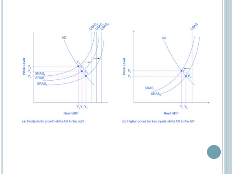
Слайд 11How productivity growth shifts the AS curve
Over time, productivity grows so
A higher level of productivity shifts the SRAS curve to the right because with improved productivity, firms can produce a greater quantity of output at every price level.

Слайд 13Summary
The aggregate demand/aggregate supply model is a model that shows what determines total
Movements of either the aggregate supply or aggregate demand curve in an AD/AS diagram will result in a different equilibrium output and price level.
The aggregate supply curve shifts to the right as productivity increases or the price of key inputs falls, making a combination of lower inflation, higher output, and lower unemployment possible.
The aggregate supply curve shifts to the left as the price of key inputs rises, making a combination of lower output, higher unemployment, and higher inflation possible.
When an economy experiences stagnant growth and high inflation at the same time it is referred to as stagflation.

Слайд 14How do changes by consumers and firms affect AD?
When consumers feel
Consumer and business confidence often reflect macroeconomic realities. For example, confidence is usually high when the economy is growing briskly and low during a recession. However, economic confidence can sometimes rise or fall due to factors that do not have a close connection to the immediate economy, like a risk of war, election results, foreign policy events, or a pessimistic prediction about the future by a prominent public figure.

Слайд 15Government macroeconomic policy choices can shift AD.
Take, for example, government spending–one

Слайд 16During a recession, when unemployment is high and many businesses are
The original equilibrium during the recession is at point E0 relatively far from the full-employment level of output. The tax cut, by increasing consumption, shifts the AD curve to the right. At the new equilibrium E1 real GDP rises and unemployment falls and – because in this diagram the economy has not yet reached its potential or full-employment level of GDP – any rise in the price level remains muted.

Слайд 17Summary
The aggregate demand/aggregate supply model is a model that shows what determines total
The aggregate demand curve shifts to the right as the components of aggregate demand–consumption spending, investment spending, government spending, and spending on exports minus imports–rise. The AD curve will shift back to the left as these components fall.
AD components can change because of different personal choices–like those resulting from consumer or business confidence–or from policy choices like changes in government spending and taxes.
If the AD curve shifts to the right, then the equilibrium quantity of output and the price level will rise. If the AD curve shifts to the left, then the equilibrium quantity of output and the price level will fall.
Whether equilibrium output changes relatively more than the price level or whether the price level changes relatively more than output is determined by where the AD curve intersects with the AS curve.