- Главная
- Разное
- Дизайн
- Бизнес и предпринимательство
- Аналитика
- Образование
- Развлечения
- Красота и здоровье
- Финансы
- Государство
- Путешествия
- Спорт
- Недвижимость
- Армия
- Графика
- Культурология
- Еда и кулинария
- Лингвистика
- Английский язык
- Астрономия
- Алгебра
- Биология
- География
- Детские презентации
- Информатика
- История
- Литература
- Маркетинг
- Математика
- Медицина
- Менеджмент
- Музыка
- МХК
- Немецкий язык
- ОБЖ
- Обществознание
- Окружающий мир
- Педагогика
- Русский язык
- Технология
- Физика
- Философия
- Химия
- Шаблоны, картинки для презентаций
- Экология
- Экономика
- Юриспруденция
10 principles of economics презентация
Содержание
- 1. 10 principles of economics
- 2. Economy… . . . The word economy
- 3. PRINCIPLES OF ECONOMICS A household and an
- 4. PRINCIPLES OF ECONOMICS Society and Scarce Resources:
- 5. Economics Economics is the study of how
- 6. 10 PRINCIPLES OF ECONOMICS How people make
- 7. 10 PRINCIPLES OF ECONOMICS How people interact
- 8. 10 PRINCIPLES OF ECONOMICS The forces and
- 9. Principle #1: People Face Tradeoffs Trade off
- 10. Principle #1: People Face Tradeoffs To get
- 11. Principle #1: People Face Tradeoffs Efficiency v.
- 12. Principle #2: The Cost of Something Is
- 13. Principle #2: The Cost of Something Is
- 14. Principle #3: Rational People Think at the
- 15. Principle #4: People Respond to Incentives Incentives
- 16. Principle #5: Trade Can Make Everyone Better
- 17. Principle #6: Markets Are Usually a Good
- 18. Principle #6: Markets Are Usually a Good
- 19. Principle #7: Governments Can Sometimes Improve Market
- 20. Principle #7: Governments Can Sometimes Improve Market
- 21. Principle #8: The Standard of Living Depends
- 22. Principle #8: The Standard of Living Depends
- 23. Principle #9: Prices Rise When the Government
- 24. Principle #10: Society Faces a Short-run Tradeoff Between Inflation and Unemployment It’s a short-run tradeoff!
- 25. Summary When individuals make decisions, they face
- 26. Summary Trade can be mutually beneficial. Markets
- 27. Summary Productivity is the ultimate source of
- 28. Macroeconomics Introduction to Macroeconomics Zharova Liubov Zharova_l@ua.fm
- 29. Intro individual decision-making Microeconomics examines the behavior
- 30. Intro When we study the consumption behaviour
- 31. Intro Microeconomists generally conclude that markets work
- 32. Intro Macroeconomists often reflect on the microeconomic
- 33. The Roots of Macroeconomics The Great Depression
- 34. The Roots of Macroeconomics Classical economists applied
- 35. The Roots of Macroeconomics In 1936, John
- 36. Recent Macroeconomic History Fine-tuning was the phrase
- 37. Why to Study Macroeconomics? Macroeconomics is the
- 38. Macroeconomic Concerns Three of the major concerns of macroeconomics are: Inflation Output growth Unemployment
- 39. Inflation and Deflation Inflation is an increase
- 40. Inflation
- 41. Output Growth: Short Run and Long
- 42. The Business cycle is the rise and
- 43. Ups and downs of the Business Cycle
- 44. Recent Macroeconomic History Stagflation occurs when the
- 45. Stagflation Stagflation is a contraction of a
- 46. Output Growth: Short Run and Long Run
- 47. Unemployment The unemployment rate is the percentage
- 48. Unemployment
- 49. Government in the Macroeconomy There are three
- 50. Government in the Macroeconomy Fiscal policy refers
- 51. The Components of the Macroeconomy The circular
- 52. The Components of the Macroeconomy
- 53. The Components of the Macroeconomy
- 54. The Components of the Macroeconomy Transfer payments
- 55. The Three Market Arenas Households, firms, the
- 56. The Three Market Arenas Households and the
- 57. The Three Market Arenas In the money
- 58. Financial Instruments Treasury bonds, notes, and bills
- 59. The Methodology of Macroeconomics Connections to microeconomics:
- 60. Aggregate Supply and Aggregate Demand Aggregate demand
- 61. Expansion and Contraction: The Business Cycle An
- 62. Review Terms and Concepts aggregate behavior aggregate
- 63. Macroeconomics The Measurement and Structure of the National Economy Zharova Liubov Zharova_l@ua.fm
- 64. Outline National Income Accounting: The Measurement of
- 65. National Income Accounting The national income accounts
- 66. National Income Accounting Business example shows that
- 67. National Income Accounting Why are the three
- 68. National Income Accounting Some of the metrics calculated by
- 69. Gross Domestic Product The product approach to
- 70. Gross Domestic Product Market value: allows adding
- 72. GDP Newly produced: counts only things produced
- 73. GNP GNP (Gross National Product) = output
- 74. GNP Example: Engineering revenues for a road
- 75. Example If a Japanese multinational produces cars
- 76. Ratio of GNP to GDP Ukraine China
- 77. GNI GNI (Gross National Income) – measures
- 78. GNI For most nations there is little
- 79. To convert a nation’s GDP to GNI
- 82. GDP measurement The expenditure approach to measuring
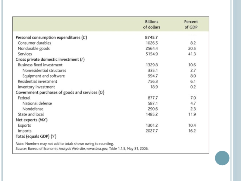
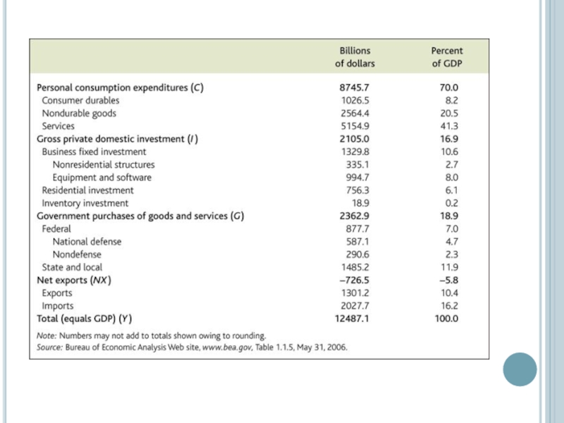
- 83. GDP measurement / expenditure approach
- 84. GDP measurement / expenditure approach
- 85. GDP measurement / expenditure approach
- 86. GDP measurement / expenditure approach
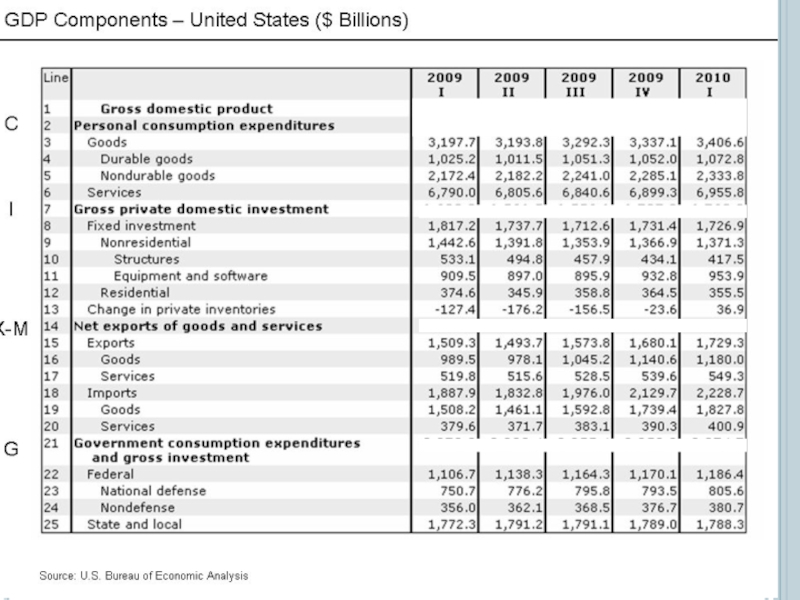
- 87. Expenditure Approach to Measuring GDP (United States)
- 88. GDP measurement / income approach
- 89. GDP measurement / income approach
- 90. Income Approach to Measuring GDP (US)
- 91. Saving and Wealth Wealth Household Wealth =
- 92. Saving and Wealth / Measures of
- 93. Saving and Wealth / Measures of
- 94. Saving and Wealth / Measures of
- 95. Saving and Wealth / Measures of
- 96. Saving and Wealth The uses of private
- 97. Saving and Wealth / Relating saving and
- 98. Saving and Wealth / Relating saving and
- 99. Saving and Wealth / Relating saving and
- 100. Measures of the Aggregate Savings
- 101. Real GDP, Price Indexes, and Inflation Real
- 102. Computers & Bicycles
- 103. Computers & Bicycles
- 104. Real GDP, Price Indexes, and Inflation Price
- 105. Real GDP, Price Indexes, and Inflation Price
- 106. Real GDP, Price Indexes, and Inflation Price
- 107. Real GDP, Price Indexes, and Inflation Inflation
- 108. Real GDP, Price Indexes, and Inflation Price
- 109. Real GDP, Price Indexes, and Inflation Price
- 110. Real GDP, Price Indexes, and Inflation Does
- 111. Interest rate Real vs. nominal interest rates
- 112. Gross National Product (GNP) Gross Domestic Product
- 113. The balance of payments, also known as
- 114. Producer Price Index (PPI) measures the average
- 115. Macroeconomics The Measurement and Structure of the National Economy Zharova Liubov Zharova_l@ua.fm
- 117. “It isn’t a case of more globalization
- 118. What Is Globalization Globalization is defined as
- 119. basic aspects of globalization In 2000, the
- 120. Globalization Encompasses Internationalization (trade & investment) Liberalization
- 121. Impact Economic impact Improvement in standard of
- 122. Focus on: Measuring globalisation STATISTICAL INDICATORS OECD
- 123. Focus on: Measuring globalisation STATISTICAL INDICATORS
- 124. Focus on: Measuring globalisation COMPOSITE INDEXES The
- 125. The A. T Kearney/FOREIGN POLICY Globalization Index (Ukraine 39)
- 126. CSGR Globalisation Index
- 127. KOF Globalization Index - 100 most globalized countries 2017
- 128. Methodology
- 129. Methodology
- 130. Methodology POLITICAL GLOBALIZATION [27%] Embassies in Country (25%) Membership
- 131. “Arguably no other place on earth has
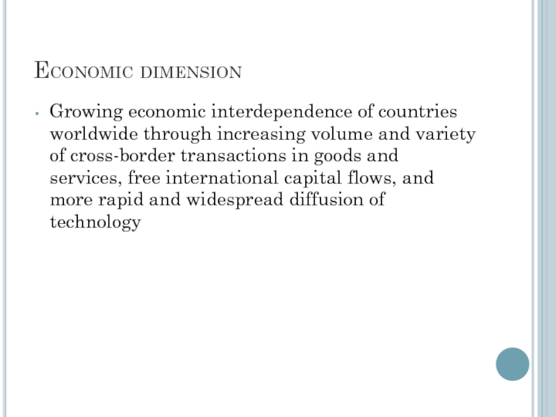
- 132. Economic dimension Growing economic interdependence of countries
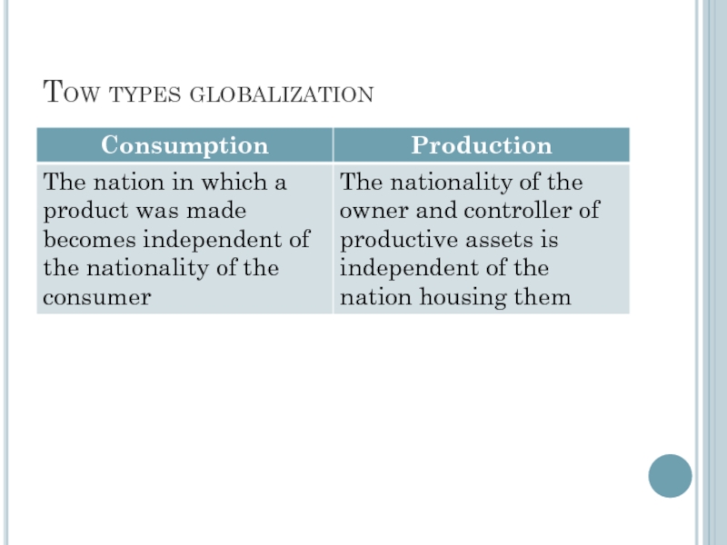
- 133. Tow types globalization
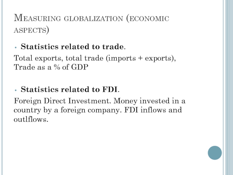
- 134. Measuring globalization (economic aspects) Statistics related to
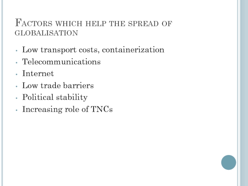
- 135. Factors which help the spread of globalisation
- 136. Increased competition among nations For example, many
- 137. Increased competition among nations “They (economists) predict
- 138. Widening income gap For example, with improved
- 139. Pros and Cons of Globalization Free trade
- 140. Pros & Cons According to supporters globalization
- 141. Pros & Cons Socially we have become
- 142. Pros & Cons The general complaint about
- 143. Pros & Cons Workers in developed countries
- 144. Pros & Cons The anti-globalists also claim
- 145. Documentory
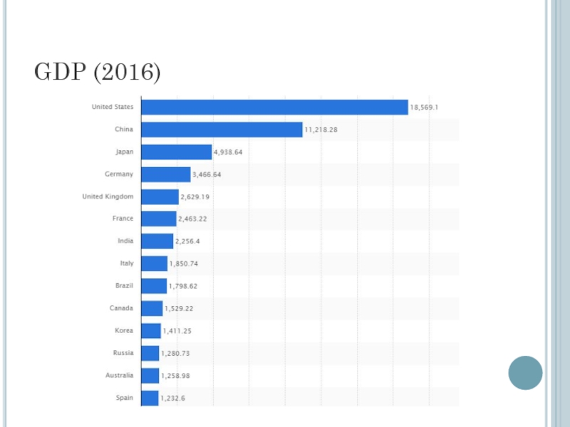
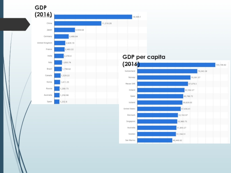
- 146. GDP (2016)
- 147. GDP per capita (2016)
- 148. Macroeconomics Productivity, Output & Employment Zharova Liubov Zharova_l@ua.fm
- 149. How much does the economy produce? The
- 150. Factors affecting productivity Technology Inputs Labor
- 151. The production function The quantity of inputs
- 152. Empirical example: US production function Studies show
- 153. Calculating “A”
- 154. Shape of the production function We can
- 155. Shape of the production function
- 156. Shape of the production function: Properties The
- 157. Effect of increasing 1000 units of capital
- 158. Marginal productivity The previous example shows that
- 159. Formal Definitions of Marginal Productivity Marginal Productivity
- 160. Changes in the production function The production
- 161. Demand for labor In contrast to the
- 162. Determination of the demand for labor Demand
- 163. Determination of demand for labor To maximize
- 164. Determination of labor demand w* N*
- 165. Factors that shift labor demand curve Changes
- 166. Shift of the labor demand curve A
- 167. Supply of labor We have seen that
- 168. Labor supply curve Labor supply curve looks
- 169. Factors that shift the labor supply curve Left Left Right Right
- 170. Labor market equilibrium w* MPN
- 171. When profit maximizing wage is higher than
- 172. Effects of adverse supply shock W2 N2
- 173. What if all workers are not alike?
- 174. Unemployment: the untold story of full-employment Full-employment
- 175. Productivity / GDP per capita & GDP (PPP) Prof. Zharova Liubov Zharova_l@ua.fm
- 176. GDP Per Capita / GDP PPP (purchasing
- 177. Why do we need GDP per capita?
- 178. GDP (2016) GDP per capita (2016)
- 179. Why do we need GDP per capita?
- 180. The most productive countries (2015) NB: Working
- 182. Labour productivity Labour productivity is defined as
- 184. Labour productivity and utilization Labour productivity growth
- 186. Multifactor productivity Multifactor productivity (MFP) reflects the
- 188. What Is Purchasing Power Parity? Macroeconomic analysis
- 189. PPP calculation Problem: To make a comparison
- 190. The Big Mac Index: an example of
- 192. GDP with PPP Example: One way to
- 193. Transport Costs: Goods that are not available
- 194. Venezuela case
- 195. From the 10 years of military dictatorship
- 196. By 1950, as the rest of the
- 197. The Downfall of Venezuela’s Economy From 1950
- 199. Although oil revenues are tempting to rely
- 200. The graphic shows Venezuela’s oil revenues (in
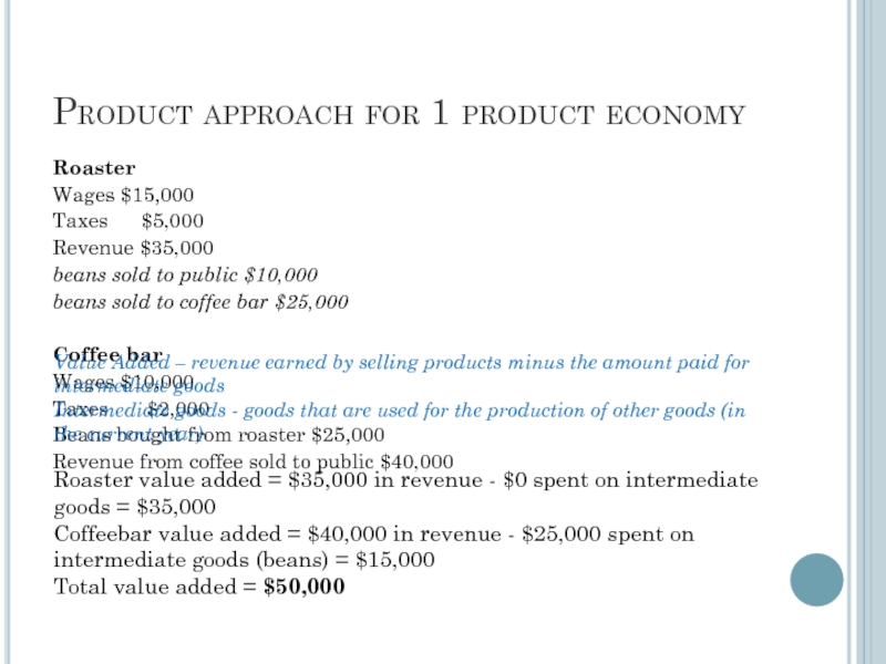
- 201. Nicolás Maduro, who took over after the
- 202. The details of today’s crisis and intense
- 203. Macroeconomics Consumption, Savings & Investment Zharova Liubov Zharova_l@ua.fm
- 204. Consumption Consumption can be defined in different
- 205. Theories of Consumption Keynes mentioned several subjective
- 206. S. Kuznets vision Contrary to Keynes’s
- 208. Relative Income Theory of Consumption (J.S. Duesenberry)
- 209. Demonstration Effect: individuals or households try to
- 210. Ratchet Effect - when income of individuals
- 211. Life Cycle Theory of Consumption ( Albert Ando & Franco Modigliani)
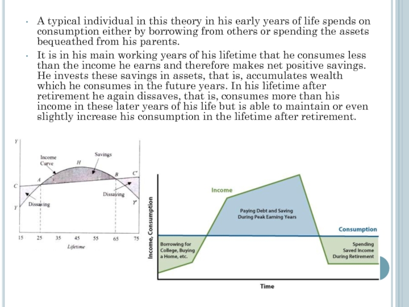
- 212. A typical individual in this theory in
- 213. Shortcomings: criticized the assumption of life cycle
- 214. Permanent Income Theory of Consumption (Milton Friedman)
- 215. Relationship between Consumption and Permanent Income: Cp
- 216. In addition to permanent income (Yp), the
- 217. Conclusions: Permanent income hypothesis is similar
- 218. Real income vs. nominal income The term
- 219. Savings Savings, according to Keynesian economics, consists of
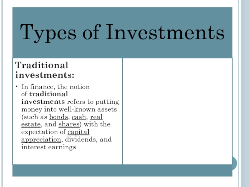
- 221. Investments Definition: Money committed or property acquired
- 222. Leverage Firms (Companies), are the best place
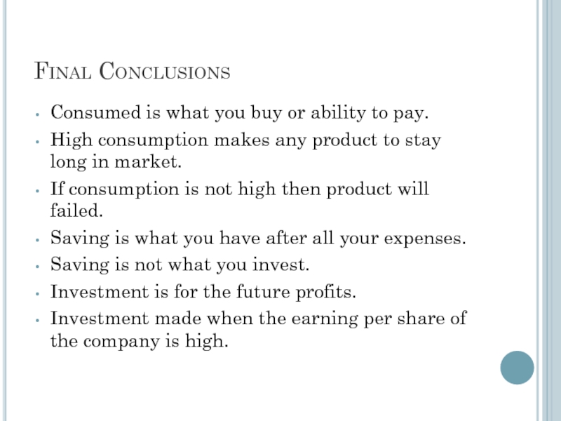
- 224. Final Conclusions Consumed is what you buy
- 225. Macroeconomics GDP Income Economic Growth Zharova Liubov
- 226. GDP = is the monetary value of
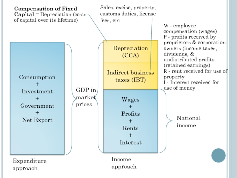
- 227. Approaches to calculate GDP Expenditure & Income
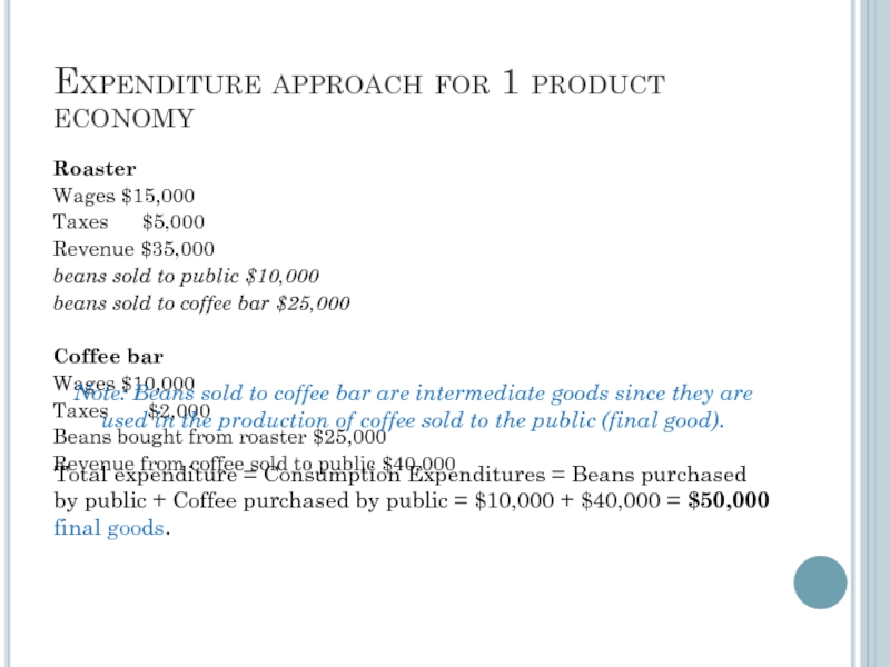
- 236. Expenditure approach for 1 product economy Roaster
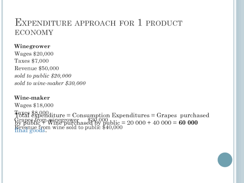
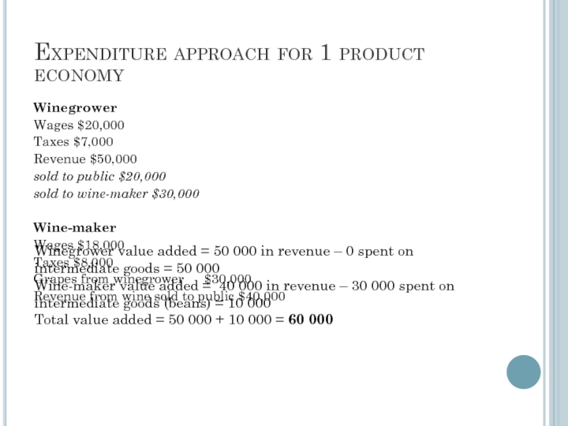
- 237. Expenditure approach for 1 product economy Winegrower
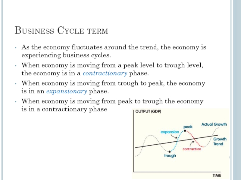
- 238. Product approach GDP is the sum of
- 239. Product approach for 1 product economy Roaster
- 240. Expenditure approach for 1 product economy Winegrower
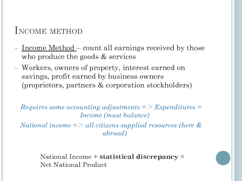
- 241. Income method Income Method – count all
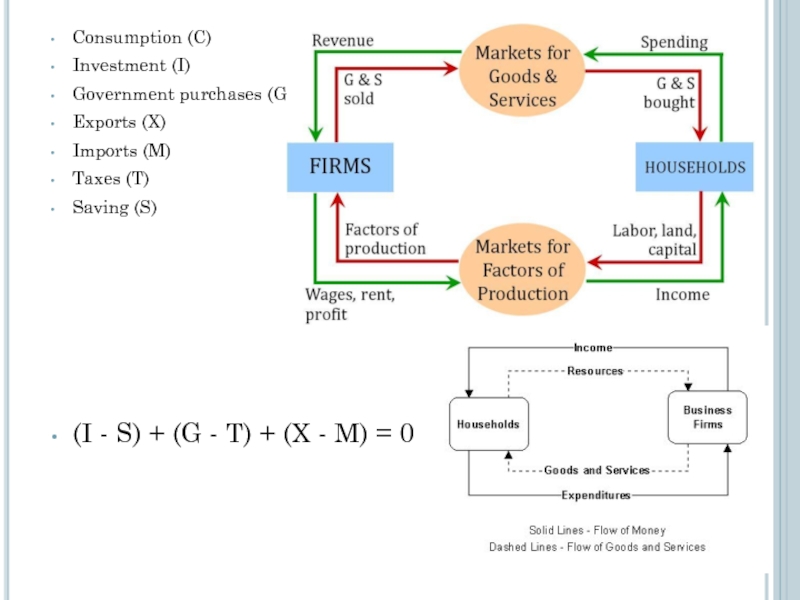
- 242. Consumption (C) Investment (I) Government purchases (G)
- 243. Consumption + Investment + Government + Net
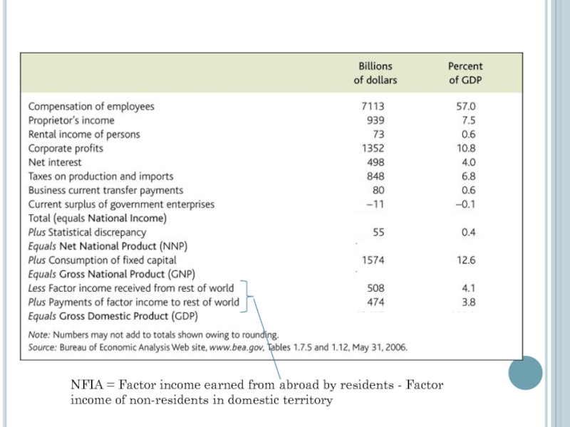
- 244. NFIA = Factor
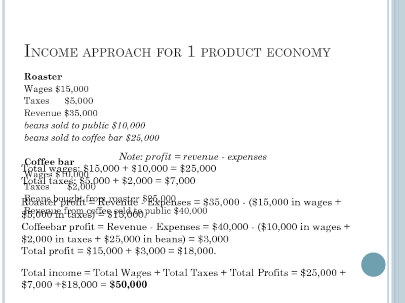
- 246. Income approach for 1 product economy Roaster
- 247. Income approach for 1 product economy Winegrower
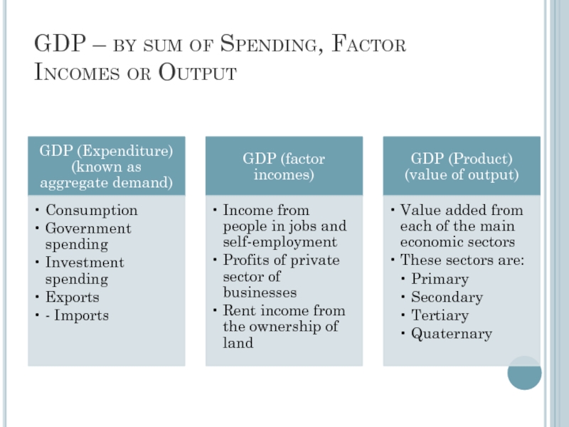
- 248. GDP – by sum of Spending, Factor Incomes or Output
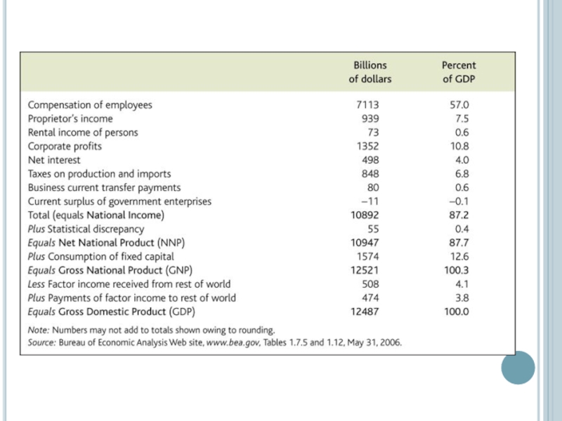
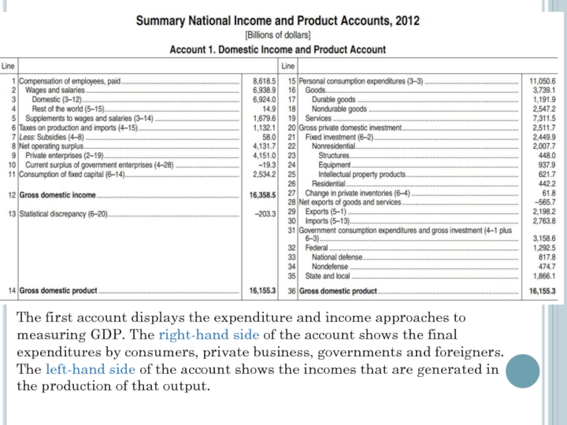
- 249. The first account displays the expenditure and
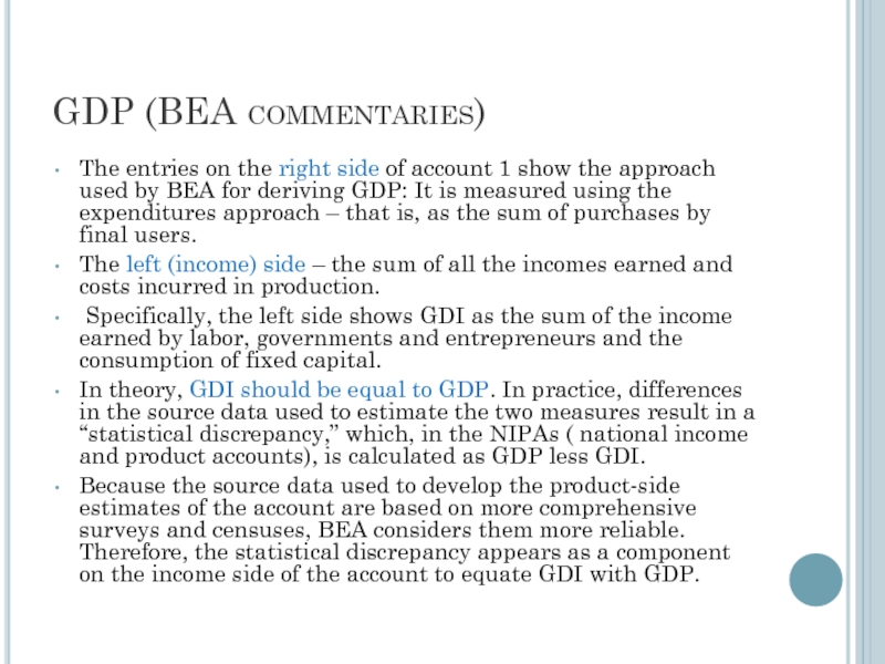
- 250. GDP (BEA commentaries) The entries on the
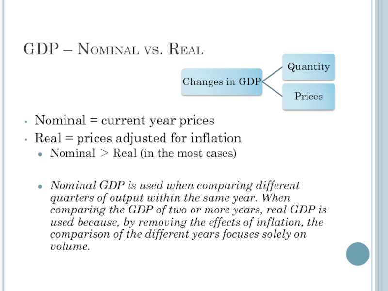
- 252. GDP – Nominal vs. Real Nominal =
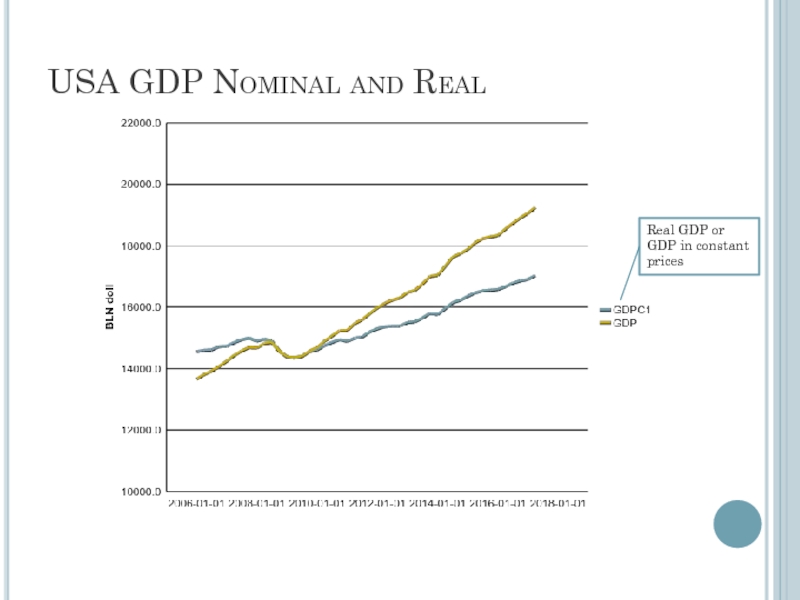
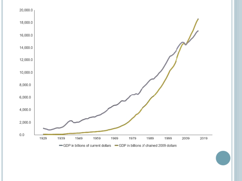
- 253. USA GDP Nominal and Real Real GDP or GDP in constant prices
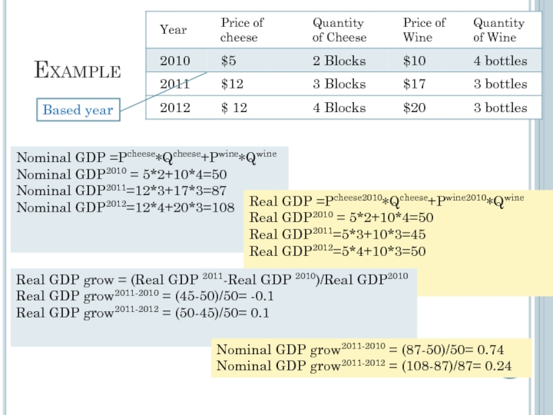
- 255. Example Nominal GDP =Pcheese∗QCheese+Pcheese∗QCheese Nominal GDP =Pcheese∗Qcheese+Pwine∗Qwine
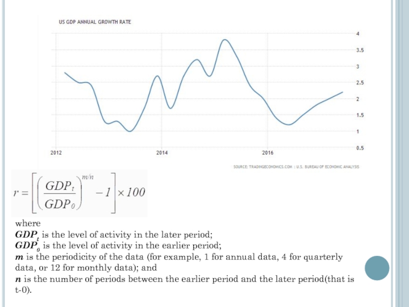
- 256. where GDPt is the level of activity in
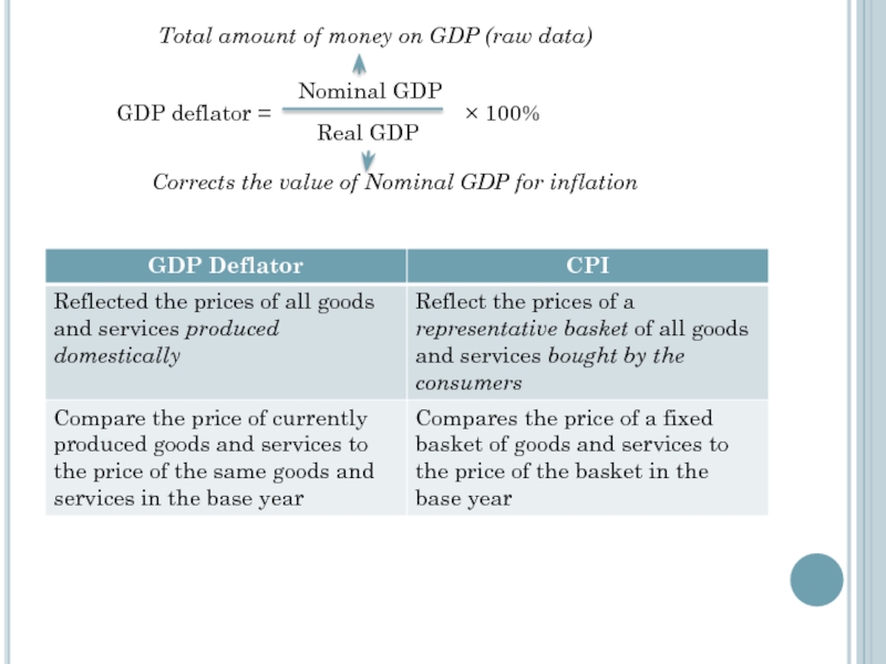
- 257. Deflator GDP GDP deflator is an index
- 258. GDP deflator = Nominal GDP Real GDP
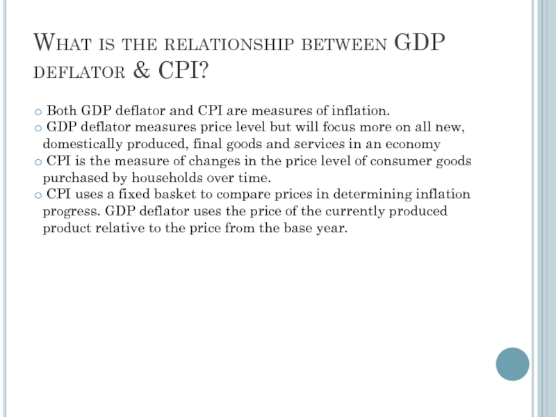
- 259. What is the relationship between GDP deflator
- 260. Malaysia
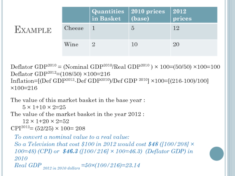
- 261. Example The value of this market basket
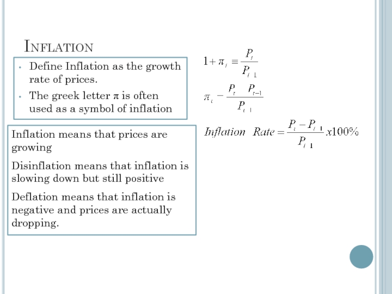
- 262. Define Inflation as the growth rate of
- 263. Macroeconomics GDP /Business Cycle Unemployment Zharova Liubov
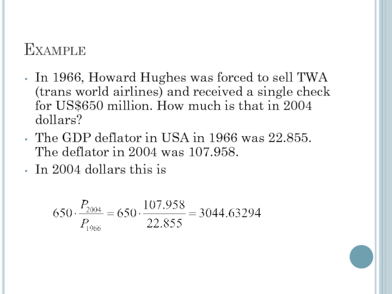
- 264. Example In 1966, Howard Hughes was forced
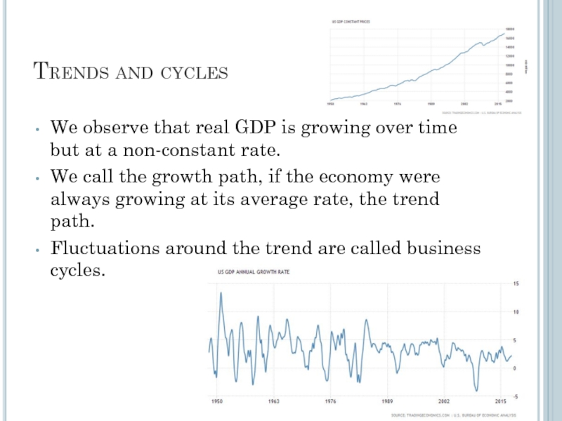
- 265. Trends and cycles We observe that real
- 266. Business Cycle term As the economy fluctuates
- 267. The correlation of business cycles implies that
- 268. North American Free Trade Agreement (NAFTA) It
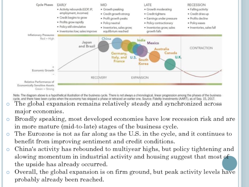
- 269. The global expansion remains relatively steady and
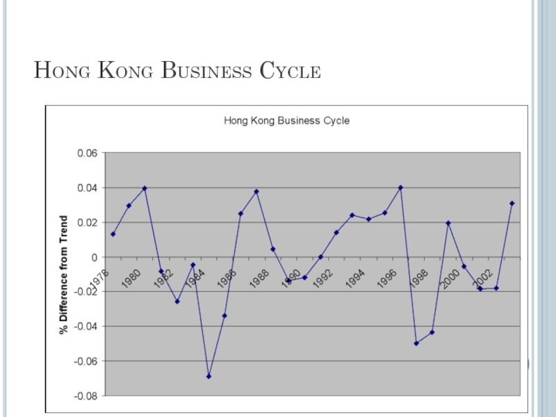
- 270. Recession and booms Business cycle positions are
- 271. Hong Kong Business Cycle
- 272. Business Cycles & Co-movement Business cycles
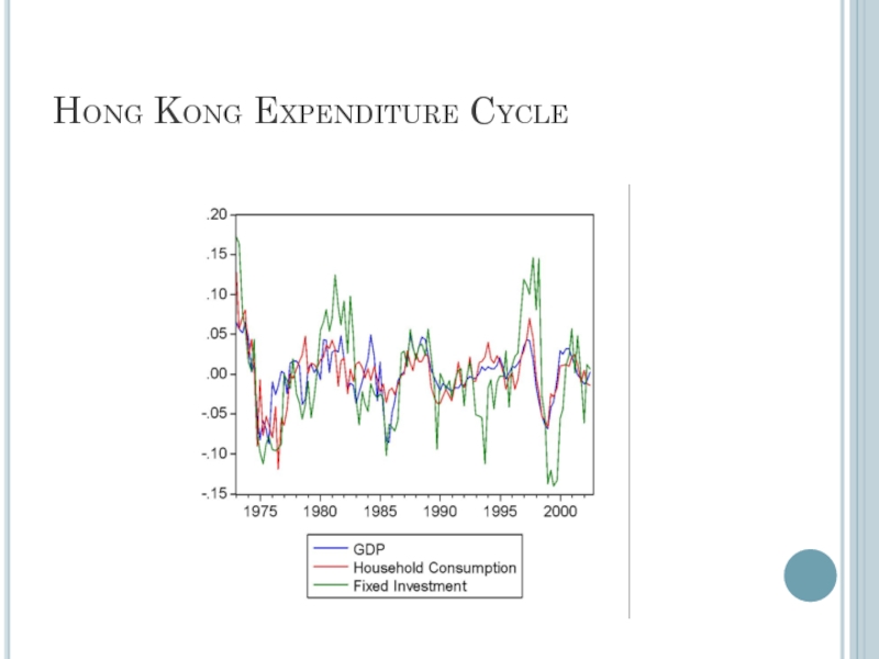
- 273. Business Cycles & Sub-Categories Expenditure. Consumption and
- 274. Hong Kong Expenditure Cycle
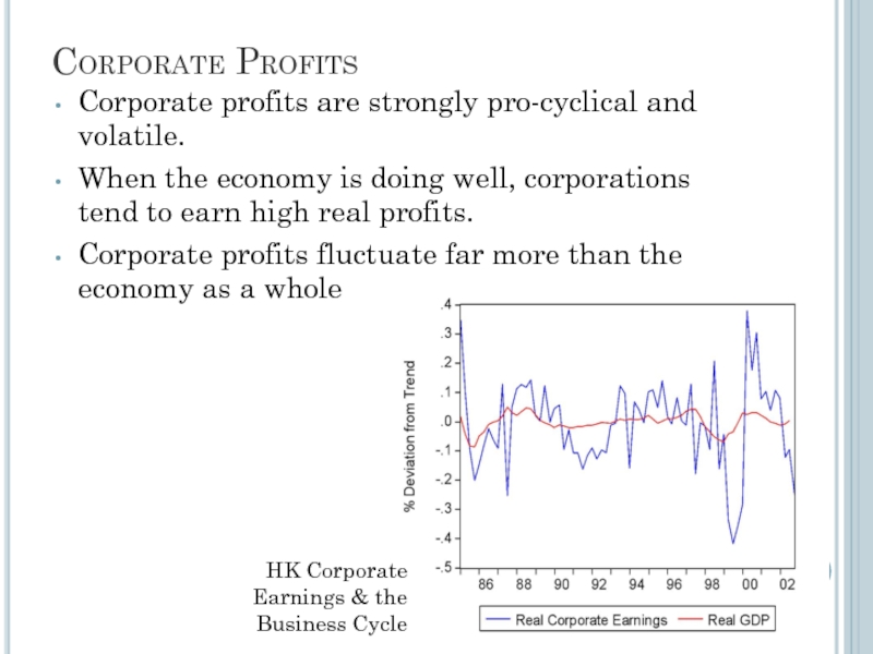
- 275. Corporate Profits Corporate profits are strongly pro-cyclical
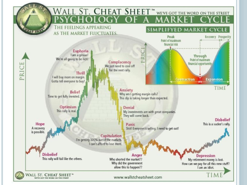
- 276. Using financial market data to predict business
- 277. The traditional business cycle frequency is around
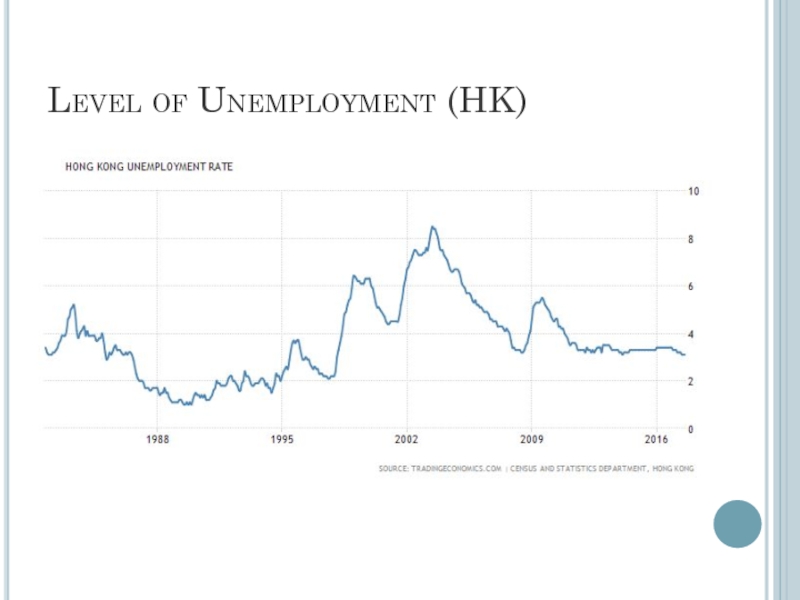
- 279. Level of Unemployment (HK)
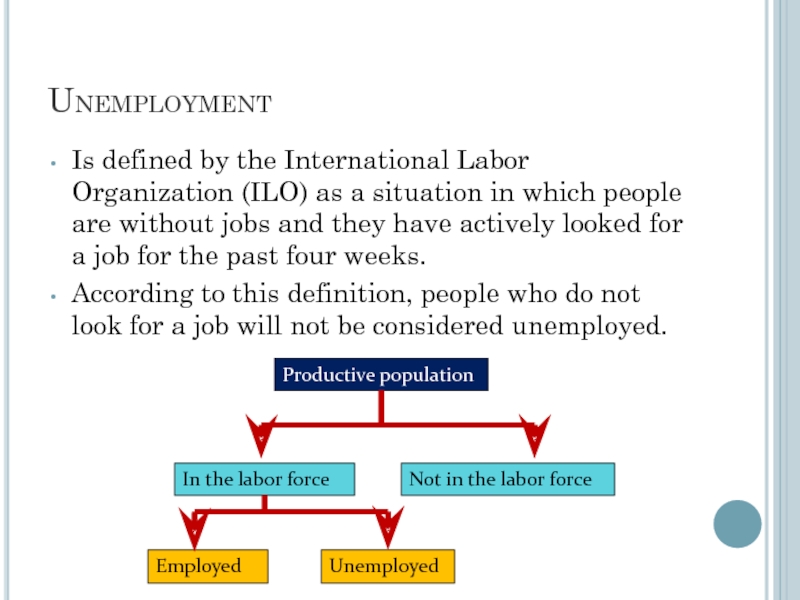
- 280. Unemployment Is defined by the International Labor
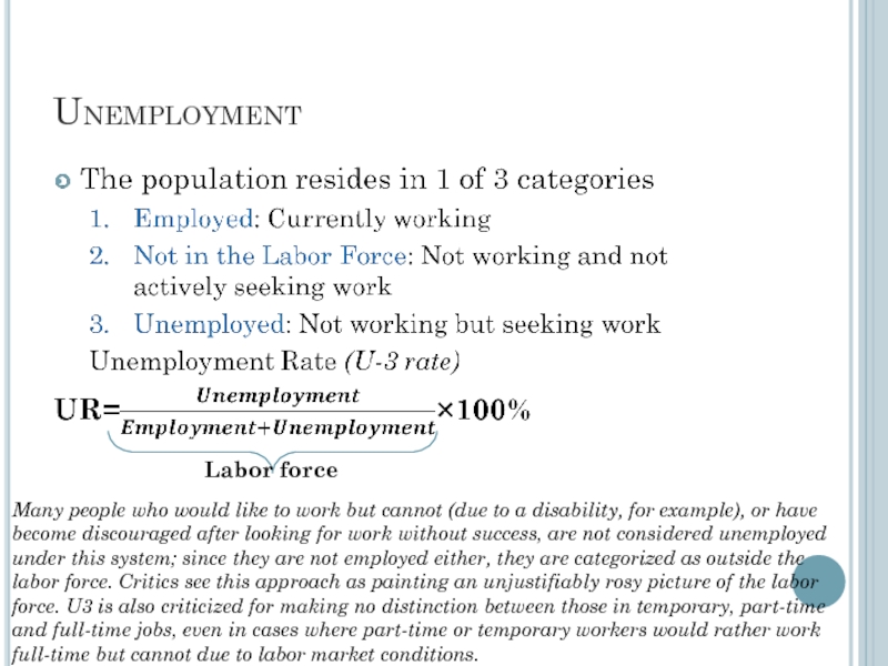
- 281. Unemployment Labor force Many people
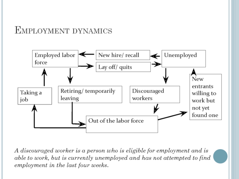
- 282. Employment dynamics Employed labor force Unemployed
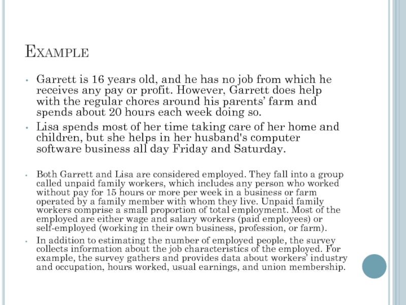
- 283. Example Who is counted as employed? On
- 284. Example Garrett is 16 years old, and
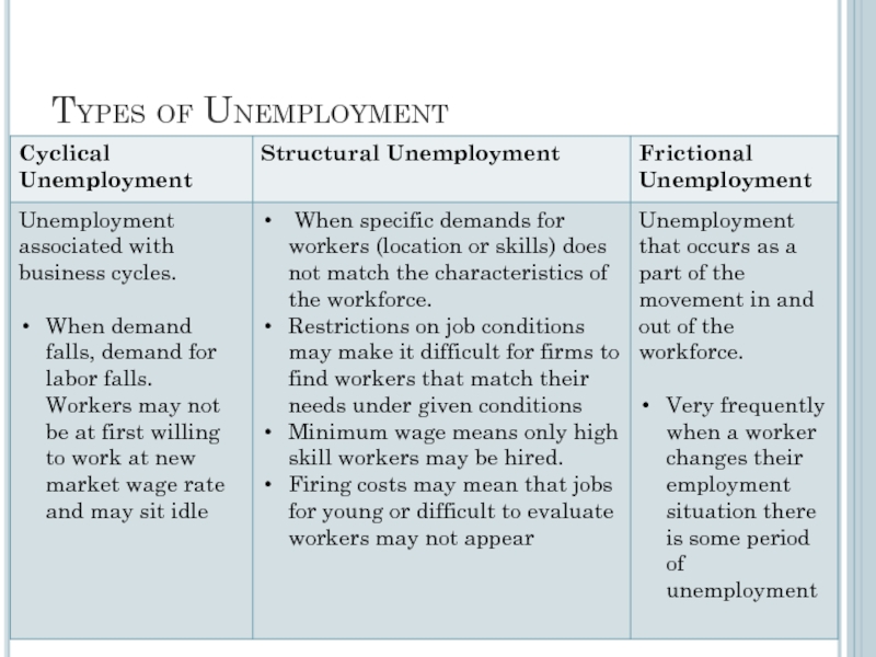
- 285. Types of Unemployment
- 286. Underemployment Underemployment is a measure of employment
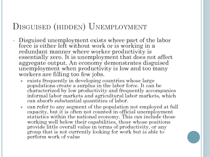
- 287. Disguised (hidden) Unemployment Disguised unemployment exists where
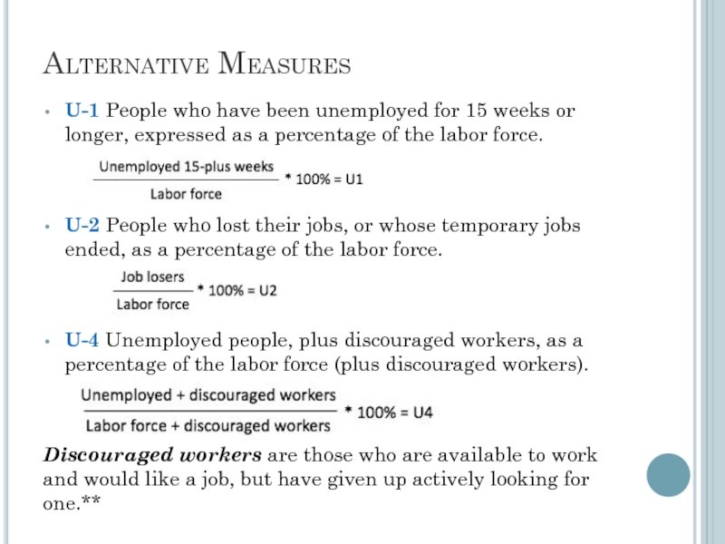
- 288. Alternative Measures U-1 People who have been
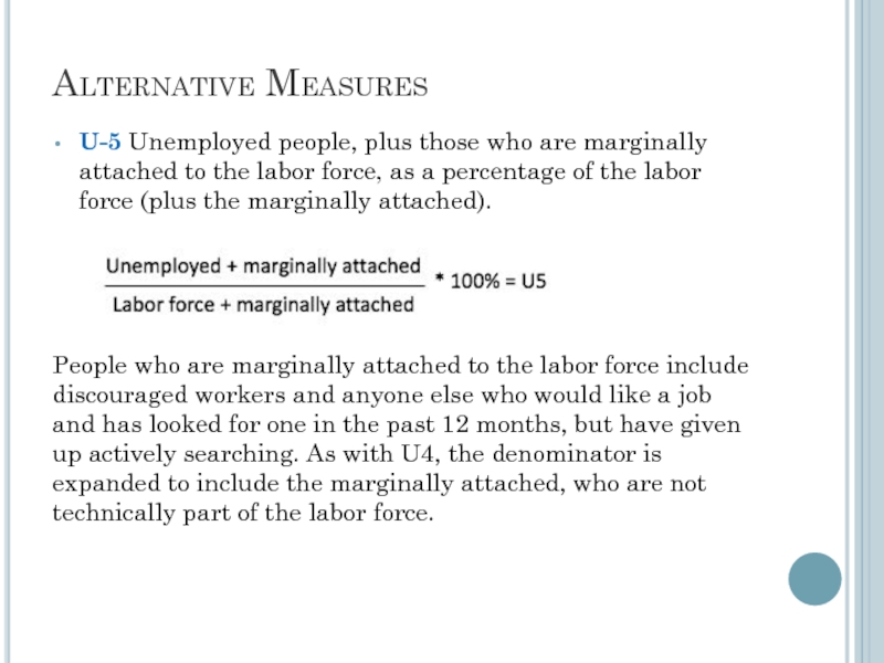
- 289. Alternative Measures U-5 Unemployed people, plus those
- 290. Alternative Measures U-6 Unemployed people, plus people
- 292. Tightly regulated labor markets increase structural unemployment.
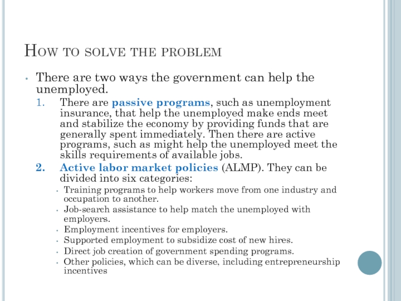
- 293. How to solve the problem There are
- 294. Macroeconomics aggregated supply and demand Zharova Liubov
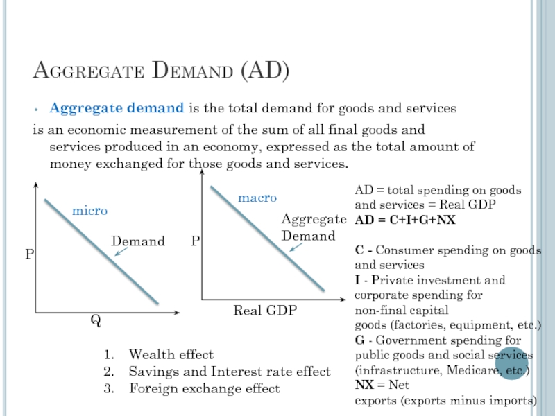
- 295. Aggregate Demand (AD) Aggregate demand is the
- 296. AD shifts AD = C+I+G+NX change in
- 297. Components of AS Consumer goods. Private consumer goods
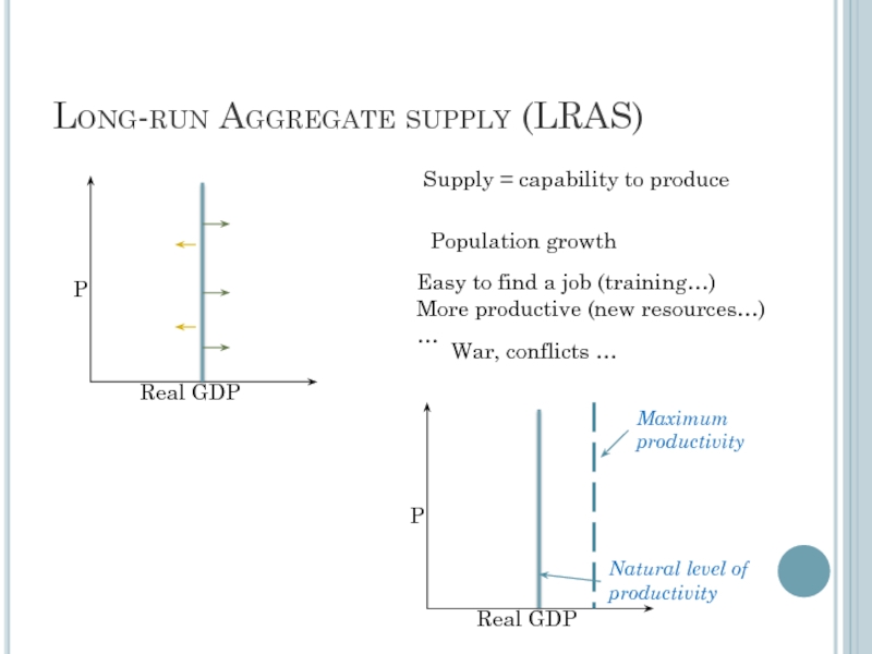
- 298. Long-run Aggregate supply (LRAS) Supply = capability
- 299. Sort-run Aggregate Supply (SRAS) Rising the price
- 300. Summirising Aggregate supply is the total quantity of
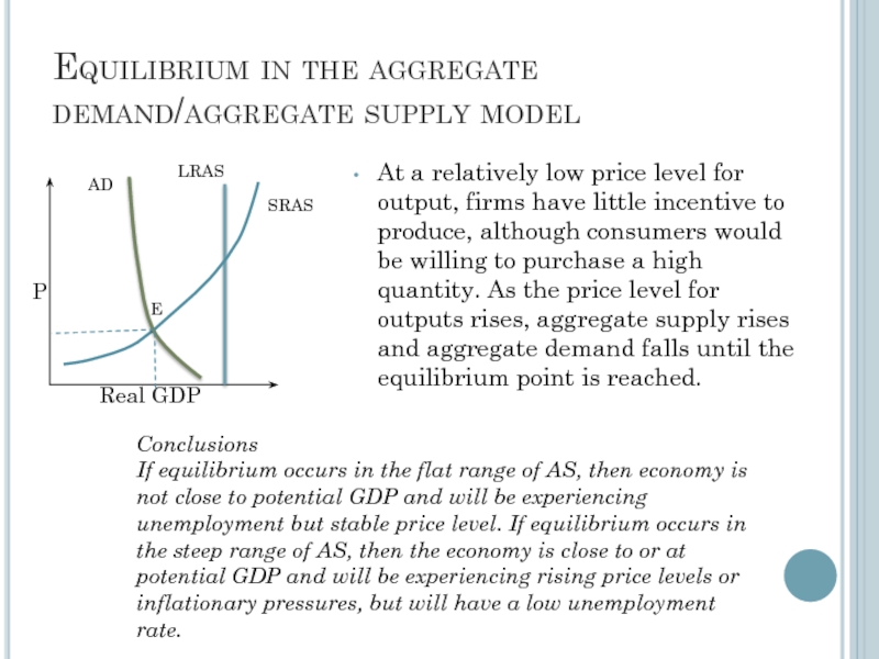
- 301. Equilibrium in the aggregate demand/aggregate supply model
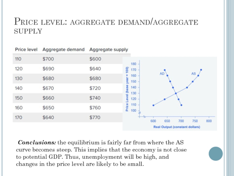
- 302. Price level: aggregate demand/aggregate supply Conclusions: the
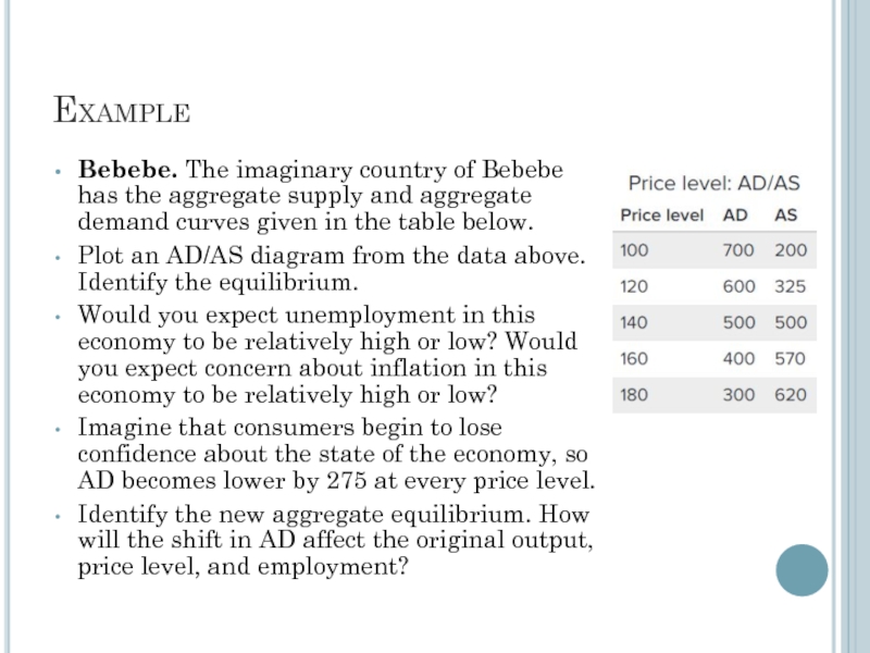
- 303. Example Bebebe. The imaginary country of Bebebe
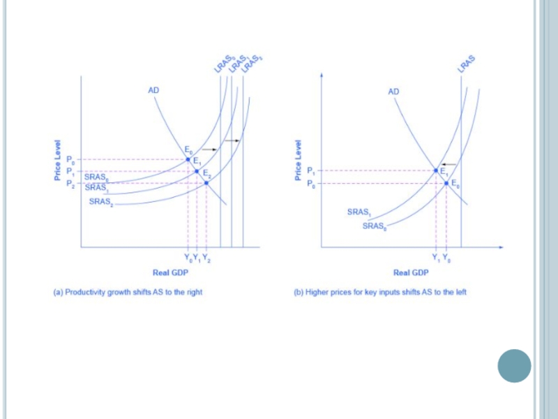
- 304. How productivity growth shifts the AS curve
- 306. Summary The aggregate demand/aggregate supply model is a model
- 307. How do changes by consumers and firms
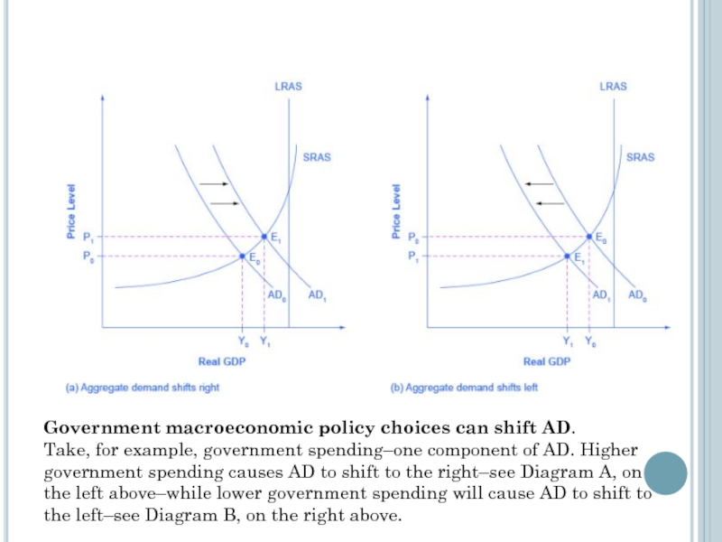
- 308. Government macroeconomic policy choices can shift AD.
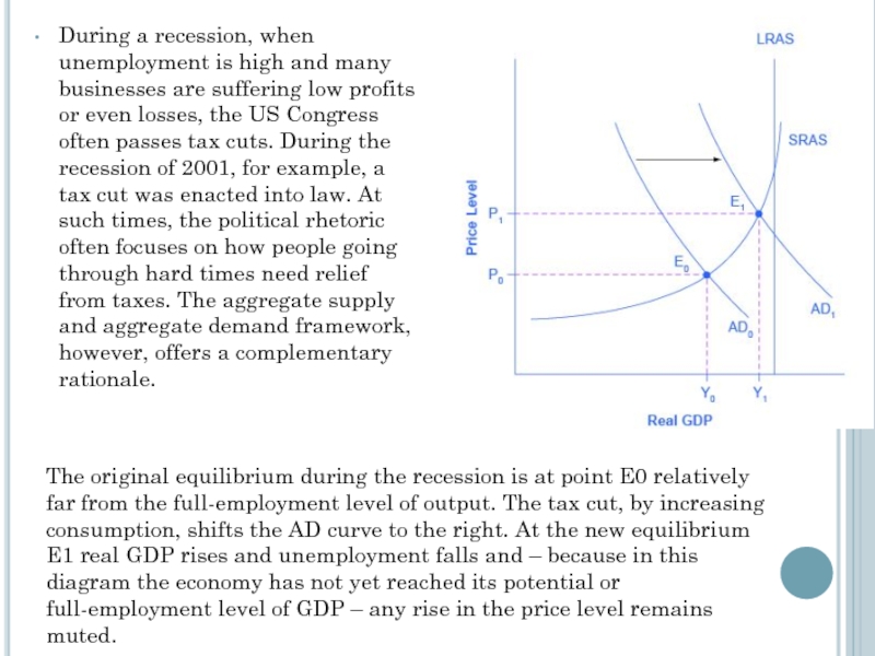
- 309. During a recession, when unemployment is high
- 310. Summary The aggregate demand/aggregate supply model is a model
Слайд 3PRINCIPLES OF ECONOMICS
A household and an economy face many decisions:
Who will
What goods and how many of them should be produced?
What resources should be used in production?
At what price should the goods be sold?
Слайд 4PRINCIPLES OF ECONOMICS
Society and Scarce Resources:
The management of society’s resources is
Scarcity. . . means that society has limited resources and therefore cannot produce all the goods and services people wish to have.
Слайд 5Economics
Economics is the study of how society manages its scarce resources.
The
Слайд 610 PRINCIPLES OF ECONOMICS
How people make decisions.
People face tradeoffs.
The cost of
Rational people think at the margin.
People respond to incentives.
Слайд 710 PRINCIPLES OF ECONOMICS
How people interact with each other.
Trade can make
Markets are usually a good way to organize economic activity.
Governments can sometimes improve economic outcomes.
Слайд 810 PRINCIPLES OF ECONOMICS
The forces and trends that affect how the
The standard of living depends on a country’s production.
Prices rise when the government prints too much money.
Society faces a short-run tradeoff between inflation and unemployment.
Слайд 9Principle #1: People Face Tradeoffs
Trade off is a situation that involves
“There is no such thing as a free lunch!”
Слайд 10Principle #1: People Face Tradeoffs
To get one thing, we usually have
Food v. clothing
Leisure time v. work
Efficiency v. equity
Making decisions requires trading off one goal against another
Слайд 11Principle #1: People Face Tradeoffs
Efficiency v. Equity
Efficiency means society gets the
Equity means the benefits of those resources are distributed fairly among the members of society.
Слайд 12Principle #2: The Cost of Something Is What You Give Up
Decisions require comparing costs and benefits of alternatives.
Whether to go to college or to work?
Whether to study or go out on a date?
Whether to go to class or sleep in?
The opportunity cost of an item is what you give up to obtain that item.
Слайд 13Principle #2: The Cost of Something Is What You Give Up
Cricketing god Sachin Tendulkar decided to quit his education in order to play professional cricket for his country.
LA Laker basketball star Kobe Bryant chose to skip college and go straight from high school to the pros where he has earned millions of dollars.
Слайд 14Principle #3: Rational People Think at the Margin
Rational people people who
Marginal changes are small, incremental adjustments to an existing plan of action.
People make decisions by comparing costs and benefits at the margin
Слайд 15Principle #4: People Respond to Incentives
Incentives – something that induces a
Marginal changes in costs or benefits motivate people to respond.
The decision to choose one alternative over another occurs when that alternative’s marginal benefits exceed its marginal costs!
Слайд 16Principle #5: Trade Can Make Everyone
Better Off
People gain from their ability
Competition results in gains from trading.
Trade allows people to specialize in what they do best.
Слайд 17Principle #6: Markets Are Usually a Good Way to Organize Economic
A market economy is an economy that allocates resources through the decentralized decisions of many firms and households as they interact in markets for goods and services.
Households decide what to buy and who to work for.
Firms decide who to hire and what to produce
Слайд 18Principle #6: Markets Are Usually a Good Way to Organize Economic
Adam Smith made the observation that households and firms interacting in markets act as if guided by an “invisible hand.”
Because households and firms look at prices when deciding what to buy and sell, they unknowingly take into account the social costs of their actions.
As a result, prices guide decision makers to reach outcomes that tend to maximize the welfare of society as a whole.
Слайд 19Principle #7: Governments Can Sometimes Improve Market Outcomes
Market failure occurs when
When the market fails (breaks down) government can intervene to promote efficiency and equity
Слайд 20Principle #7: Governments Can Sometimes Improve Market Outcomes
Market failure may be
an externality, which is the impact of one person or firm’s actions on the well-being of a bystander.
market power, which is the ability of a single person or firm to unduly influence market prices.
Слайд 21Principle #8: The Standard of Living Depends on a Country’s Production
Standard
By comparing personal incomes.
By comparing the total market value of a nation’s production.
Слайд 22Principle #8: The Standard of Living Depends on a Country’s Production
Almost
Productivity is the amount of goods and services produced from each hour of a worker’s time.
Standard of living may be measured in different ways:
By comparing personal incomes.
By comparing the total market value of a nation’s production.
Слайд 23Principle #9: Prices Rise When the
Government Prints Too Much Money
Inflation is
One cause of inflation is the growth in the quantity of money.
When the government creates large quantities of money, the value of the money falls.
Слайд 24Principle #10: Society Faces a Short-run
Tradeoff Between Inflation and Unemployment
It’s a
Слайд 25Summary
When individuals make decisions, they face tradeoffs among alternative goals.
The cost
Rational people make decisions by comparing marginal costs and marginal benefits.
People change their behavior in response to the incentives they face.
Слайд 26Summary
Trade can be mutually beneficial.
Markets are usually a good way of
Government can potentially improve market outcomes if there is some market failure or if the market outcome is inequitable
Слайд 27Summary
Productivity is the ultimate source of living standards.
Money growth is the
Society faces a short-run tradeoff between inflation and unemployment.
Слайд 29Intro
individual decision-making Microeconomics examines the behavior of units—business firms and households.
Macroeconomics
Aggregate behavior refers to the behavior of all households and firms together.
Слайд 30Intro
When we study the consumption behaviour or equilibrium of a consumer;
we study a UNIT and not the SYSTEM in which it is operating
Слайд 31Intro
Microeconomists generally conclude that markets work well.
Macroeconomists, however, observe that some
Sticky prices are prices that do not always adjust rapidly to maintain the equality between quantity supplied and quantity demanded.
Слайд 32Intro
Macroeconomists often reflect on the microeconomic principles underlying macroeconomic analysis, or
Слайд 33The Roots of Macroeconomics
The Great Depression was a period of severe
Stock Markets crashed!
9000 banks filed for bankruptcy
Banks that survived stopped giving loans.
People cut down spending
Large amounts of inventories started piling up
Businesses stopped production….layoffs!( 25% unemployment)
Purchasing power declined
Hawley – Smoot tariff imposed on imports in 1930
Decline in world trade & economic retaliation.
Слайд 34The Roots of Macroeconomics
Classical economists applied microeconomic models, or “market clearing”
However, simple classical models failed to explain the prolonged existence of high unemployment during the Great Depression. This provided the impetus for the development of macroeconomics
Слайд 35The Roots of Macroeconomics
In 1936, John Maynard Keynes published The General
Keynes believed governments could intervene in the economy and affect the level of output and employment.
During periods of low private demand, the government can stimulate aggregate demand to lift the economy out of recession.
Слайд 36Recent Macroeconomic History
Fine-tuning was the phrase used by Walter Heller to
The use of Keynesian policy to fine-tune the economy in the 1960s, led to disillusionment in the 1970s and early 1980s.
Слайд 37Why to Study Macroeconomics?
Macroeconomics is the study of the nation’s economy
We can use macroeconomic analysis to:
Understand why economies grow.
Understand economic fluctuations.
Make informed business decisions.
Слайд 38Macroeconomic Concerns
Three of the major concerns of macroeconomics are:
Inflation
Output growth
Unemployment
Слайд 39Inflation and Deflation
Inflation is an increase in the overall price level.
Hyperinflation
Hyperinflations are rare, but have been used to study the costs and consequences of even moderate inflation.
Deflation is a decrease in the overall price level. Prolonged periods of deflation can be just as damaging for the economy as sustained inflation.
Слайд 41Output Growth:
Short Run and Long Run
The business cycle is the
The main measure of how an economy is doing is aggregate output:
Aggregate output is the total quantity of goods and services produced in an economy in a given period
Слайд 42The Business cycle is the rise and fall of economic activity
Слайд 43Ups and downs of the Business Cycle
Peak: at the peak of
Contraction: A decline in the real GDP. If it falls for two consecutive quarters, it is said the economy to be in a recession.
Trough: The Low Point of the GDP, just before it begins to turn up.
Recovery: When the GDP is rising from the trough.
Expansion: when the real GDP expands beyond the recovery
Recession : two consecutive quarter declines in Real DP
Слайд 44Recent Macroeconomic History
Stagflation occurs when the overall price level rises rapidly
Слайд 45Stagflation
Stagflation is a contraction of a nation’s output accompanied by inflation
Staglation
A dramatic increase in oil prices caused the stagflation of the 1970s
Слайд 46Output Growth:
Short Run and Long Run
A recession is a period during
A prolonged and deep recession becomes a depression
Policy makers attempt not only to smooth fluctuations in output during a business cycle but also to increase the growth rate of output in the long-run.
Слайд 47Unemployment
The unemployment rate is the percentage of the labor force that
The unemployment rate is a key indicator of the economy’s health.
The existence of unemployment seems to imply that the aggregate labor market is not in equilibrium.
Why do labor markets not clear when other markets do?
Слайд 49Government in the Macroeconomy
There are three kinds of policy that the
Fiscal policy
Monetary policy
Growth or supply-side policies
Слайд 50Government in the Macroeconomy
Fiscal policy refers to government policies concerning taxes
Monetary policy consists of tools used by the Federal Reserve to control the quantity of money in the economy.
Growth policies are government policies that focus on stimulating aggregate supply instead of aggregate demand.
Слайд 51The Components of the Macroeconomy
The circular flow diagram shows the income
Everyone’s expenditure is someone else’s
receipt. Every transaction must have two sides.
Слайд 54The Components of the Macroeconomy
Transfer payments are payments made by the
Слайд 55The Three Market Arenas
Households, firms, the government, and the rest of
Goods-and-services market
Labor market
Money (financial) market
Слайд 56The Three Market Arenas
Households and the government purchase goods and services
In the labor market, firms and government purchase (demand) labor from households (supply).
The total supply of labor in the economy depends on the sum of decisions made by households.
Слайд 57The Three Market Arenas
In the money market – sometimes called the
Households supply funds to this market in the expectation of earning income, and also demand (borrow) funds from this market.
Firms, government, and the rest of the world also engage in borrowing and lending, coordinated by financial institutions.
Слайд 58Financial Instruments
Treasury bonds, notes, and bills are promissory notes issued by
Corporate bonds are promissory notes issued by corporations when they borrow money
Shares of stock are financial instruments that give to the holder a share in the firm’s ownership and therefore the right to share in the firm’s profits.
Dividends are the portion of a corporation’s profits that the firm pays out each period to its shareholders.hen they borrow money.
Слайд 59The Methodology of Macroeconomics
Connections to microeconomics:
Macroeconomic behavior is the sum of
Слайд 60Aggregate Supply and
Aggregate Demand
Aggregate demand is the total demand for goods
Aggregate supply is the total supply of goods and services in an economy.
Aggregate supply and demand curves are more complex than simple market supply and demand curves.
Слайд 61Expansion and Contraction:
The Business Cycle
An expansion, or boom, is the period
A contraction, recession, or slump is the period in the business cycle from a peak down to a trough, during which output and employment fall.
The Business cycle is the rise and fall of economic activity relative to the long-term growth trend of the economy
Слайд 62Review Terms and Concepts
aggregate behavior
aggregate demand
aggregate output
aggregate supply
business cycle
circular flow
contraction, recession,
slump
corporate bonds
deflation
depression
microeconomics
monetary policy
recession
shares of stock
stagflation
sticky prices
supply-side policies
transfer payments
Treasury bonds, notes, bills
unemployment rate
dividends
expansion or boom
fine tuning
fiscal policy
Great Depression
hyperinflation
inflation
macroeconomics
microeconomic
foundations of
macroeconomics
Слайд 63Macroeconomics
The Measurement and
Structure of the
National Economy
Zharova Liubov
Zharova_l@ua.fm
Слайд 64Outline
National Income Accounting: The Measurement of Production, Income, and Expenditure
Gross Domestic
Saving and Wealth
Real GDP, Price Indexes, and Inflation
Interest Rates
Слайд 65National Income Accounting
The national income accounts is an accounting framework used
The product approach measures the amount of output produced, excluding output used up in intermediate stages of production.
The income approach measures the incomes received by the producers of output
The expenditure approach measures the amount of
spending by the ultimate purchasers of output
Слайд 66National Income Accounting
Business example shows that all three approaches are equal
Important
Слайд 67National Income Accounting
Why are the three approaches equivalent?
They must be, by
Any output produced (product approach) is purchased by someone (expenditure approach) and results in income to someone (income approach)
The fundamental identity of national income accounting:
total production = total income = total expenditure
Слайд 68National Income Accounting
Some of the metrics calculated by using national income accounting include
Gross
Gross National Product (GNP)
Gross National Income (GNI).
Слайд 69Gross Domestic Product
The product approach to measuring GDP
GDP (gross domestic product)
2016
Слайд 70Gross Domestic Product
Market value: allows adding together unlike items by valuing
Problem: misses nonmarket items such as homemaking, the value of environmental quality, and natural resource depletion
There is some adjustment to reflect the underground economy
Government services (that aren’t sold in markets) are valued at their cost of production
Слайд 72GDP
Newly produced: counts only things produced in the given period; excludes
Final goods and services* - are those that are not intermediate
*Don’t count intermediate goods and services (those used up in the production of other goods and services in the same period that they themselves were produced)
Capital goods (goods used to produce other goods) are final goods since they aren’t used up in the same period that they are produced
Inventory investment (the amount that inventories of unsold finished goods, goods in process, and raw materials have changed during the period) is also treated as a final good
Adding up value added works well, since it automatically excludes intermediate goods
Слайд 73GNP
GNP (Gross National Product) = output produced by domestically owned factors
GDP = output produced within a nation
GDP = GNP – NFP
NFP – Net Factor Payments from abroad
Слайд 74GNP
Example: Engineering revenues for a road built by a U.S. company
Difference between GNP and GDP is small for the United States, about 0.2%, but higher for countries that have many citizens working abroad
Слайд 75Example
If a Japanese multinational produces cars in the UK, this production
If a UK firm makes a profit from insurance companies located abroad, then if this profit is returned to UK nationals, then this net income from overseas assets will be added to UK GNP.
Note, if a Japanese firm invests in the UK, it will still lead to higher GNP, as some national workers will see higher wages. However, the increase in GNP will not be as high as GDP.
If a county has similar inflows and outflows of income from assets, then GNP and GDP will be very similar.
However, if a country has many multinationals who repatriate income from local production, then GNP will be lower than GDP. For example, Luxembourg has a GDP of $87,400 but a GNP of only $45,360.
Слайд 77GNI
GNI (Gross National Income) – measures income received by a country
GNI = GDP + Net Income received from overseas
Слайд 78GNI
For most nations there is little difference between GDP and GNI
GNI
GNI can be well below GDP
Ireland, since large-scale repatriation of profits from foreign companies located there far exceeds income flows from overseas. Ireland’s GNI was 20% below its GDP, which means that although Ireland attracts substantial foreign investment that contributes to its economic growth, a big chunk of the profits arising from such foreign investment does not remain in the nation. In this case, GNI may be a better indicator of Ireland’s economic performance than GDP, since the latter overstates the strength of the Irish economy.
Слайд 79To convert a nation’s GDP to GNI
Three terms need to be
net compensation receipts,
net property income receivable
net taxes (minus subsidies) receivable on production and imports.
GDP(Canada) = $1,624.6 million
Net compensation receipts = 0
Net property income receivable = - $28.2 million
Net taxes = 0
GNI(Canada) = $1,624.6 + (-28.2) = $1,596.4 million
Слайд 82GDP measurement
The expenditure approach to measuring GDP
Measures total spending on final
Four main categories of spending: consumption (C), investment (I), Government purchases of goods and services (G), and net exports (NX)
Y = C + I + G + NX
the income-expenditure identity
exports minus imports
Слайд 83GDP measurement /
expenditure approach
Consumption: spending by domestic households on
About 2/3 of U.S. GDP
Three categories:
Consumer durables (examples: cars, TV sets, furniture, major appliances)
Nondurable goods (examples: food, clothing, fuel)
Services (examples: education, health care, financial services, transportation)
Слайд 84GDP measurement /
expenditure approach
Investment: spending for new capital goods
About 1/6 of U.S. GDP
Business (or nonresidential) fixed investment: spending by businesses on structures and equipment and software
Residential fixed investment: spending on the construction of houses and apartment buildings
Inventory investment: increases in firms’ inventory holdings
Слайд 85GDP measurement /
expenditure approach
Government purchases of goods and services:
About 1/5 of U.S. GDP
Most by state and local governments, not federal government
Not all government expenditures are purchases of goods and services
Some are payments that are not made in exchange for current goods and services
One type is transfers, including Social Security payments, welfare, and unemployment benefits
Another type is interest payments on the government debt
Some government spending is for capital goods that add to the nation’s capital stock, such as highways, airports, bridges, and water and sewer systems
Слайд 86GDP measurement /
expenditure approach
Net exports: exports minus imports
Exports: goods
Imports: goods produced abroad that are purchased by residents in the country
Imports are subtracted from GDP, as they represent goods produced abroad, and were included in consumption, investment, and government purchases
Слайд 88GDP measurement /
income approach
Adds up income generated by production
National Income = (compensation of employees (including benefits) + (proprietors’ income) + (rental income of persons) + (corporate profits) + (net interest) + (taxes on production and imports) + (business current transfer payments) + (current surplus of government enterprises)
National income + statistical discrepancy = Net National Product
Net National Product + Depreciation (the value of capital that wears out in the period) = Gross National Product (GNP)
GNP – Net Factor Payments (NFP) = GDP
Слайд 89GDP measurement /
income approach
Private sector and government sector income
Private
Y or GDP – private sector income earned at home
NFP –net factor payments from abroad
TR – payments from the government sector (transfers)
INT – interest on government debt
T – taxes paid to gouvernement
Government’s net income = Taxes – TRansfers – INTerest payments = T – TR – INT
Private disposable income + government’s net income = GDP + NFP = GNP
Слайд 91Saving and Wealth
Wealth
Household Wealth = (Household’s Assets) – (Household’s Liabilities)
National
Saving by individuals, businesses, and government determine wealth
Слайд 92Saving and Wealth /
Measures of aggregate saving
Saving = Current Income
Saving Rate = Saving / Current Income
Private Saving = Private disposable income – Consumption
Spvt = (Y + NFP – T + TR + INT) – C
Слайд 93Saving and Wealth /
Measures of aggregate saving
Government Saving = Net
Sgovt = (T – TR – INT) – G
Government saving = government budget surplus = Government Receipts – Government Outlays
Government receipts = Tax revenue (T)
Government outlays = Government purchases of goods and services (G) + TRansfers (TR) + INTerest payments on government debt (INT)
Government budget deficit = – Sgovt
Simplification: count government investment as government purchases, not investment
Слайд 94Saving and Wealth /
Measures of aggregate saving
National saving
National Saving =
S = Spvt + Sgovt =
= [Y + NFP – T + TR + INT – C] +
+[T – TR – INT – G] =
= Y + NFP – C – G =
= GNP – C – G
Слайд 95Saving and Wealth /
Measures of aggregate saving
The uses of private
S = I + (NX + NFP)
S = I + CA
Derived from
S = Y + NFP – C – G and Y = C + I + G + NX
CA = NX + NFP = current account balance
Слайд 96Saving and Wealth
The uses of private saving
Spvt = I + (–Sgovt)
(using S = Spvt + Sgovt)
The uses-of-saving identity—saving is used in three ways:
investment (I)
government budget deficit (–Sgovt)
current account balance (CA)
Слайд 97Saving and Wealth /
Relating saving and wealth
Stocks and flows
Flow variables: measured
Stock variables: measured at a point in time (quantity of money, value of houses, capital stock)
Flow variables often equal rates of change of stock variables
Wealth and saving as stock and flow (wealth is a stock, saving is a flow)
Слайд 98Saving and Wealth /
Relating saving and wealth
National wealth: domestic physical assets
Country’s domestic physical assets (capital goods and land)
Country’s net foreign assets = (Foreign assets (foreign stocks, bonds, and capital goods owned by domestic residents)) – (Foreign liabilities (domestic stocks, bonds, and capital goods owned by foreigners))
Wealth matters because the economic well-being of a country depends on it
Слайд 99Saving and Wealth /
Relating saving and wealth
National wealth: domestic physical assets
Changes in national wealth
Change in value of existing assets and liabilities (change in price of financial assets, or depreciation of capital goods)
National saving (S = I + CA) raises wealth
Comparison of U.S. saving and investment with other countries
The United States is a low-saving country; Japan is a high-saving country
U.S. investment exceeds U.S. saving, so we have a negative current-account balance
Слайд 101Real GDP, Price Indexes, and Inflation
Real GDP
Nominal variables are those in
Problem: Do changes in nominal values reflect changes in prices or quantities?
Real variables: adjust for price changes; reflect only quantity changes
Nominal GDP is the dollar value of an economy’s final output measured at current market prices
Real GDP is an estimate of the value of an economy’s final output, adjusting for changes in the overall price level
Слайд 104Real GDP, Price Indexes, and Inflation
Price Indexes
A price index measures the
GDP deflator = 100 × nominal GDP/real GDP
Note that base year P = 100
Слайд 105Real GDP, Price Indexes, and Inflation
Price Indexes
Consumer Price Index (CPI)
Price index
Слайд 106Real GDP, Price Indexes, and Inflation
Price Indexes
GDP
Choice of expenditure base period
BEA (Bureau of Economic Analysis) compromised by developing chain-weighted GDP
Now, however, components of real GDP don’t add up to real GDP, but discrepancy is usually small
Слайд 107Real GDP, Price Indexes, and Inflation
Inflation
Calculate inflation rate:
inflation rate for the
GDP deflator 2015 = 1
GDP deflator 2016 = 1,5
Inflation rate = (1.5-1.0)/1 = 0.5
Слайд 108Real GDP, Price Indexes, and Inflation
Price Indexes
Does CPI inflation overstate increases
The Boskin Commission reported that the CPI was biased upwards by as much as one to two percentage points per year
One problem is that adjusting the price measures for changes in the quality of goods is very difficult
A consumer price index (CPI) measures changes in the price level of a market basket of consumer goods and services purchased by households
Слайд 109Real GDP, Price Indexes, and Inflation
Price Indexes
Does CPI inflation overstate increases
Price indexes with fixed sets of goods don’t reflect substitution by consumers when one good becomes relatively cheaper than another
This problem is known as substitution bias
Слайд 110Real GDP, Price Indexes, and Inflation
Does CPI inflation overstate increases in
If inflation is overstated, then real incomes are higher than we thought and we’ve over indexed payments like Social Security
Latest research suggests bias is still 1% per year or higher
Слайд 111Interest rate
Real vs. nominal interest rates
Interest rate: a rate of return
Real interest rate: rate at which the real value of an asset increases over time
Nominal interest rate: rate at which the nominal value of an asset increases over time
The expected real interest rate
If ,
real interest rate = expected real interest rate
Слайд 112Gross National Product (GNP) Gross Domestic Product (GDP) Net National Product (NNP) Net National
Gross National Product (GNP) is the total value of final goods and services produced in a year by domestically owned factors of production
Gross Domestic Product (GDP) is the total value of final goods and services produced within a country's borders in a year
NNP equals the GDP minus depreciation on a country's capital goods
NNP – Indirect Taxes = Net National Income (NNI), it encompasses the income of households, businesses, and the government. It can be expressed as:
NNI = C + I + G + (NX) + net foreign factor income - indirect taxes - depreciation
Слайд 113The balance of payments, also known as balance of international payments
The current account shows the net amount a country is earning if it is in surplus, or spending if it is in deficit
The capital account records the net change in ownership of foreign assets
The IMF definition of Balance of Payment
Слайд 114Producer Price Index (PPI) measures the average changes in prices received
It is one of several price indexes
Consumer price index
Producer price index
Export price index
Import price index
GDP deflator
Слайд 115Macroeconomics
The Measurement and
Structure of the
National Economy
Zharova Liubov
Zharova_l@ua.fm
Слайд 117“It isn’t a case of more globalization or less, but of
Pier Carlo Padoan, Italy’s Finance Minister
Слайд 118What Is Globalization
Globalization is defined as a process that, based on
economic globalization
cultural globalization
political globalization
Слайд 119basic aspects of globalization
In 2000, the International Monetary Fund (IMF) identified
trade and transactions,
capital and investment movements,
migration and movement of people,
the dissemination of knowledge.
Environmental challenges (global warming, cross-boundary water and air pollution, and overfishing of the ocean)
Слайд 120Globalization Encompasses
Internationalization (trade & investment)
Liberalization (freeing markets)
Universalization (cultural interchange)…or…
Westernization (Western cultural
“Deterritorialization” (the severance of social, political, or cultural practices from their native places and populations)
Слайд 121Impact
Economic impact
Improvement in standard of living
Increased competition among nations
Widening income gap
Social impact
Increased awareness of foreign cultures
Loss of local culture
Environmental impact
Environmental degradation
Environmental management
Слайд 122Focus on: Measuring globalisation
STATISTICAL INDICATORS
OECD Economic Globalization Indicators helps identify the
World Development Indicators (WDI). The WDI affords readers more than 900 indicators organized in six sections: World View, People, Environment, Economy, States and Markets, and Global Links. In each section a plethora of information is presented. ndencies within OECD countries.
Слайд 123Focus on: Measuring globalisation
STATISTICAL INDICATORS
UNCTAD Development and Globalization: Facts and
Global Policy Forum (GPF) gathers a large number of tables and graphs providing the main features of globalization, asking what is new, what drives the process, how it changes politics, and how it affects global institutions like UN. In addition to indicators of social and economic policy, trade and capital flows, global poverty and development etc.
Слайд 124Focus on: Measuring globalisation
COMPOSITE INDEXES
The A. T Kearney/FOREIGN POLICY Globalization Index
Centre for the Study of Globalisation and Regionalisation (CSGR) Globalisation Index (2004 – the last data)
Konjunkturforschungsstelle (KOF) Swiss Economic Institute Index of Globalization (2017 – the last data)
Слайд 130Methodology
POLITICAL GLOBALIZATION [27%]
Embassies in Country (25%)
Membership in International Organizations (27%)
Participation in U.N. Security Council
International Treaties (26%)
Слайд 131“Arguably no other place on earth has so engineered itself to
Singapore a 'canary in the gold mine of globalization’
Straits Times, May 24 2014
Слайд 132Economic dimension
Growing economic interdependence of countries worldwide through increasing volume and
Слайд 134Measuring globalization (economic aspects)
Statistics related to trade.
Total exports, total trade
Statistics related to FDI.
Foreign Direct Investment. Money invested in a country by a foreign company. FDI inflows and outlflows.
Слайд 135Factors which help the spread of globalisation
Low transport costs, containerization
Telecommunications
Internet
Low
Political stability
Increasing role of TNCs
Слайд 136Increased competition among nations
For example, many companies have shifted their production
Benefiting from the increased revenue, these countries are able to rapidly develop their infrastructure such as road networks and industrial parks, which further increased their attractiveness to foreign investors.
This poses a strong challenge for developed economies like Singapore and Taiwan and more so for less developed countries with poor infrastructure and political stability such as Cambodia and East Timor
Слайд 137Increased competition among nations
“They (economists) predict that increased competition from low-wage
World Health Organization
Слайд 138Widening income gap
For example, with improved communications and transportation, business owners
This inevitably leads to higher retrenchment rates and loss of income among the average workers, which translates into the rich getting richer and the poor becoming poorer
Слайд 139Pros and Cons of Globalization
Free trade is supposed to reduce barriers
The proponents say globalization represents free trade which promotes global economic growth; creates jobs, makes companies more competitive, and lowers prices for consumers.
Competition between countries is supposed to drive prices down. In many cases this is not working because countries manipulate their currency to get a price advantage.
It also provides poor countries, through infusions of foreign capital and technology, with the chance to develop economically and by spreading prosperity, creates the conditions in which democracy and respect for human rights may flourish. This is an ethereal goal which hasn’t been achieved in most countries
Слайд 140Pros & Cons
According to supporters globalization and democracy should go hand
There is now a worldwide market for companies and consumers who have access to products of different countries.
Gradually there is a world power that is being created instead of compartmentalized power sectors. Politics is merging and decisions that are being taken are actually beneficial for people all over the world. This is simply a romanticized view of what is actually happening.
There is more influx of information between two countries, which do not have anything in common between them.
There is cultural intermingling and each country is learning more about other cultures.
Since we share financial interests, corporations and governments are trying to sort out ecological problems for each other.
Слайд 141Pros & Cons
Socially we have become more open and tolerant towards
Most people see speedy travel, mass communications and quick dissemination of information through the Internet as benefits of globalization.
Labor can move from country to country to market their skills. (but this can cause problems with the existing labor and downward pressure on wages).
Sharing technology with developing nations will help them progress (true for small countries but stealing technologies and IP have become a big problem with larger competitors like China).
Transnational companies investing in installing plants in other countries provide employment for the people in those countries often getting them out of poverty.
Globalization has given countries the ability to agree to free trade agreements like NAFTA, South Korea Korus, and The TPP.
Слайд 142Pros & Cons
The general complaint about globalization is that it has
Globalization is supposed to be about free trade where all barriers are eliminated but there are still many barriers. For instance161 countries have value added taxes (VATs) on imports which are as high as 21.6% in Europe. The U.S. does not have VAT.
The biggest problem for developed countries is that jobs are lost and transferred to lower cost countries.” According to conservative estimates by Robert Scott of the Economic Policy Institute, granting China most favored nation status drained away 3.2 million jobs, including 2.4 million manufacturing jobs. He pegs the net losses due to our trade deficit with Japan ($78.3 billion in 2013) at 896,000 jobs, as well as an additional 682,900 jobs from the Mexico –U.S. trade-deficit run-up from 1994 through 2010.”
Слайд 143Pros & Cons
Workers in developed countries like the US face pay-cut
Large multi-national corporations have the ability to exploit tax havens in other countries to avoid paying taxes.
Multinational corporations are accused of social injustice, unfair working conditions (including slave labor wages, living and working conditions), as well as lack of concern for environment, mismanagement of natural resources, and ecological damage.
Multinational corporations, which were previously restricted to commercial activities, are increasingly influencing political decisions. Many think there is a threat of corporations ruling the world because they are gaining power, due to globalization.
Building products overseas in countries like China puts our technologies at risk of being copied or stolen, which is in fact happening rapidly
Слайд 144Pros & Cons
The anti-globalists also claim that globalization is not working
Some experts think that globalization is also leading to the incursion of communicable diseases. Deadly diseases like HIV/AIDS are being spread by travelers to the remotest corners of the globe.
Globalization has led to exploitation of labor. Prisoners and child workers are used to work in inhumane conditions. Safety standards are ignored to produce cheap goods. There is also an increase in human trafficking.
Social welfare schemes or “safety nets” are under great pressure in developed countries because of deficits, job losses, and other economic ramifications of globalization.
Слайд 149How much does the economy produce?
The quantity that an economy will
The quantity of inputs utilized in the production process and
The PRODUCTIVITY of the inputs
An economy’s productivity is basic to determining living standards.
In this lecture we shall see how productivity affects people’s incomes by helping to determine how many workers are employed and how much they receive.
Among all the inputs for production, labor is usually considered the most important input.
Therefore, first we shall study the factors that determine demand and supply of labor and then the forces that bring the labor market into equilibrium.
Equilibrium in the labor market determines wages and employment; and the level of employment together with other inputs and the level of productivity determines how much output en economy produces.
Слайд 150Factors affecting productivity
Technology
Inputs
Labor
Capital
Land
Raw materials
Machinery
Power
Time period
Слайд 151The production function
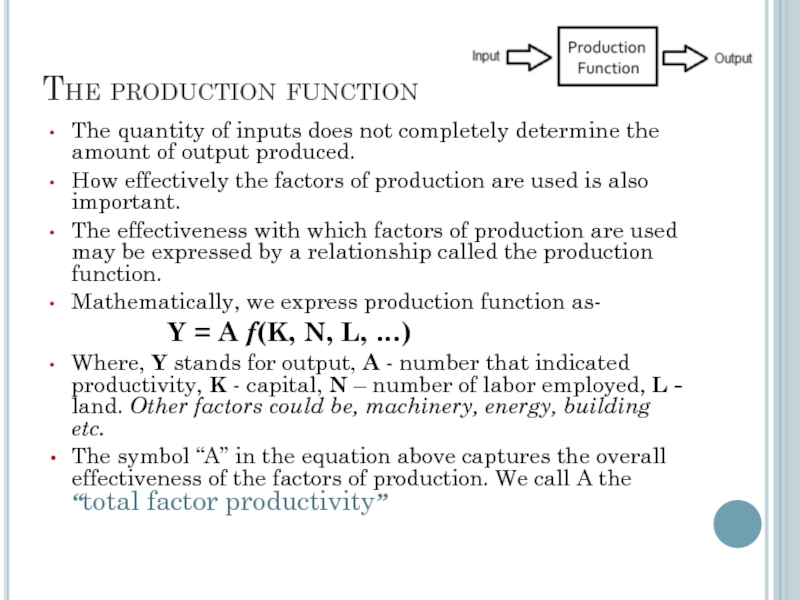
The quantity of inputs does not completely determine the
How effectively the factors of production are used is also important.
The effectiveness with which factors of production are used may be expressed by a relationship called the production function.
Mathematically, we express production function as-
Y = A f(K, N, L, …)
Where, Y stands for output, A - number that indicated productivity, K - capital, N – number of labor employed, L - land. Other factors could be, machinery, energy, building etc.
The symbol “A” in the equation above captures the overall effectiveness of the factors of production. We call A the “total factor productivity”
Слайд 152Empirical example: US production function
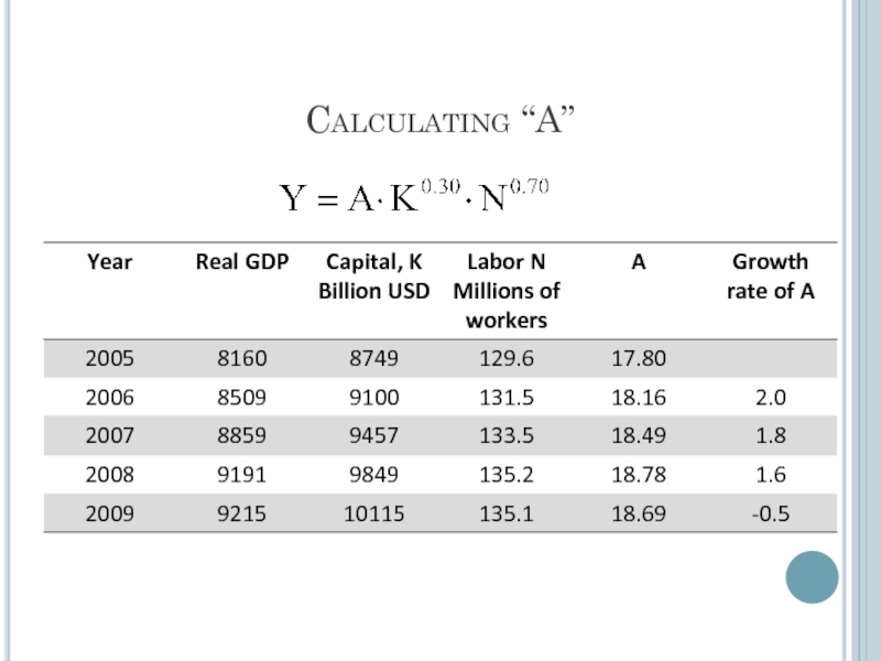
Studies show that the relationship between outputs
This type of production function is called the Cobb-Douglas production function.
Historical GDP data of US for the period 1899 – 1922 showed that the production function for US followed the form:
Слайд 154Shape of the production function
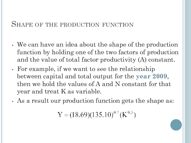
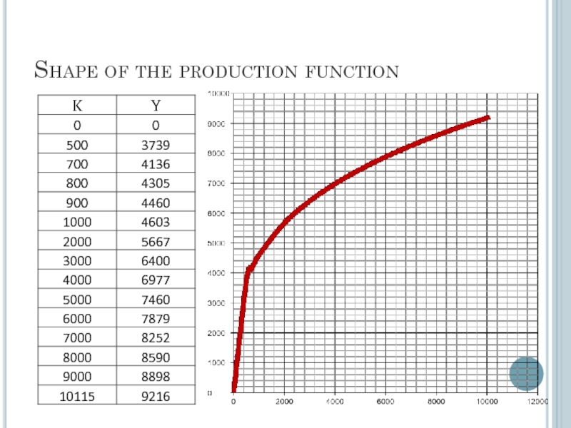
We can have an idea about the
For example, if we want to see the relationship between capital and total output for the year 2009, then we hold the values of A and N constant for that year and treat K as variable.
As a result our production function gets the shape as:
Слайд 156Shape of the production function: Properties
The production function slopes upward from
The slope of the production function becomes flatter from left to right: this means that although more capital always leads to more output, it does so at a decreasing rate.
Слайд 157Effect of increasing 1000 units of capital each time
Marginal Product of
Marginal product of capital between
K = 2000 and 3000
What is the marginal product of capital between K = 4000 and 5000? Is it less than the previous one? What does it mean?
577
483
419
373
337
309
317
Слайд 158Marginal productivity
The previous example shows that marginal productivity is falling as
Generally, when amount of labor is high compared to the amount of capital, marginal productivity of capital is high. Alternatively, when amount of labor is low compared to the amount of capital, marginal productivity of labor is high
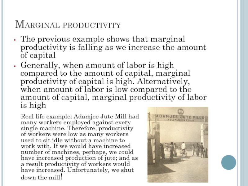
Real life example: Adamjee Jute Mill had many workers employed against every single machine. Therefore, productivity of workers were low as many workers used to sit idle without a machine to work with. If we would have increased number of machines, perhaps, we could have increased production of jute; and as a result productivity of workers would have increased. Unfortunately, we shut down the mill!
Слайд 159Formal Definitions of Marginal Productivity
Marginal Productivity of Capital: means additional output
Marginal Productivity of Labor: means additional output produced by each additional unit of labor.
Because of diminishing marginal productivity for both labor and capital the slope of production function becomes flatter from left to right.
If the marginal productivity were increasing, slope of the production function would become steeper from left to right.
If the marginal productivity were constant, the slope would be constant and the shape of the curve of production function would be a straight line.
Слайд 160Changes in the production function
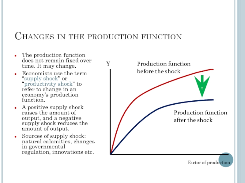
The production function does not remain fixed
Economists use the term “supply shock” or “productivity shock” to refer to change in an economy’s production function.
A positive supply shock raises the amount of output, and a negative supply shock reduces the amount of output.
Sources of supply shock: natural calamities, changes in governmental regulation, innovations etc.
Production function before the shock
Production function after the shock
Y
Factor of production
Слайд 161Demand for labor
In contrast to the amount of capital, the amount
Thus, year-to-year changes in production can be traced to the changes in employment.
Demand for labor determines the level of employment.
For this reason, understanding demand for labor is important.
To understand demand for labor we shall make the following assumptions to keep things simple:
Workers are alike
Firms have to pay competitive wage to hire workers
Firms objective is to maximize profit
Слайд 162Determination of the demand for labor
Demand for labor is determined based
Example: Suppose, wage rate (W) of labor is 80 per/day.
Слайд 163Determination of demand for labor
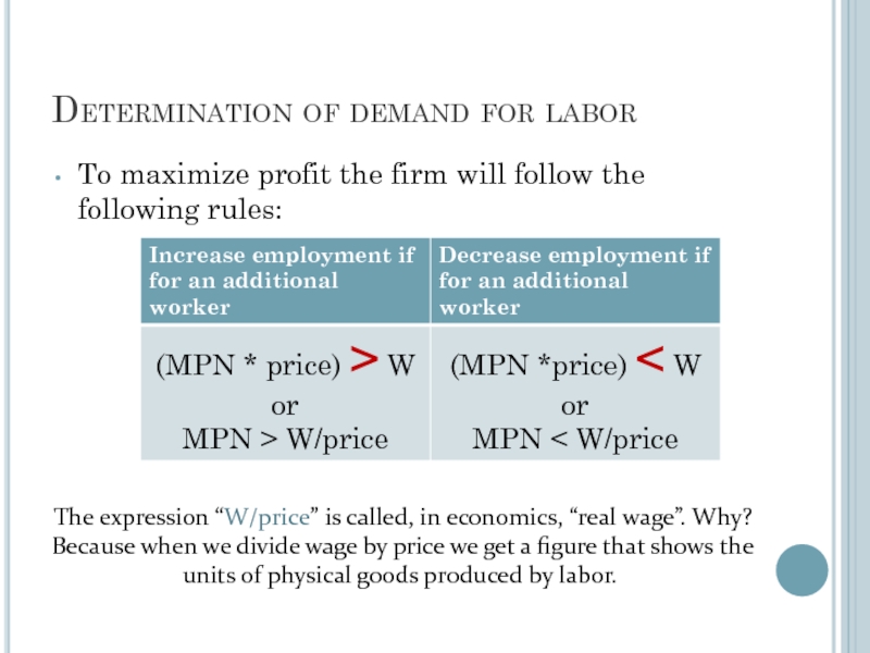
To maximize profit the firm will follow
The expression “W/price” is called, in economics, “real wage”. Why?
Because when we divide wage by price we get a figure that shows the units of physical goods produced by labor.
Слайд 164Determination of labor demand
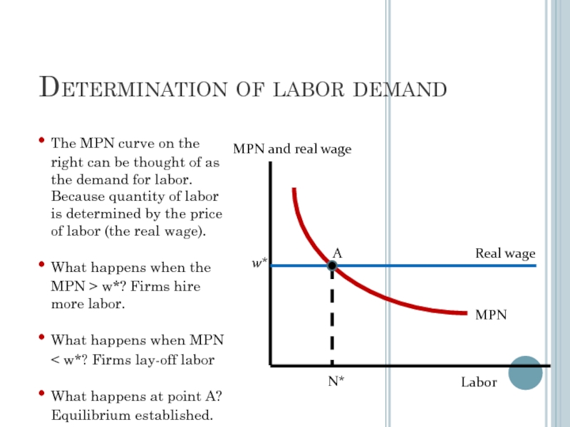
w*
N*
MPN and real wage
Labor
MPN
Real wage
The MPN curve on
What happens when the MPN > w*? Firms hire more labor.
What happens when MPN < w*? Firms lay-off labor
What happens at point A? Equilibrium established.
A
Слайд 165Factors that shift labor demand curve
Changes in the wage do not
Factors that shift labor demand curve would be something that will change the demand for labor at any given wage.
A beneficial shock will shift the labor demand curve to the right.
An adverse shock will shift the labor demand curve to the left.
Слайд 166Shift of the labor demand curve
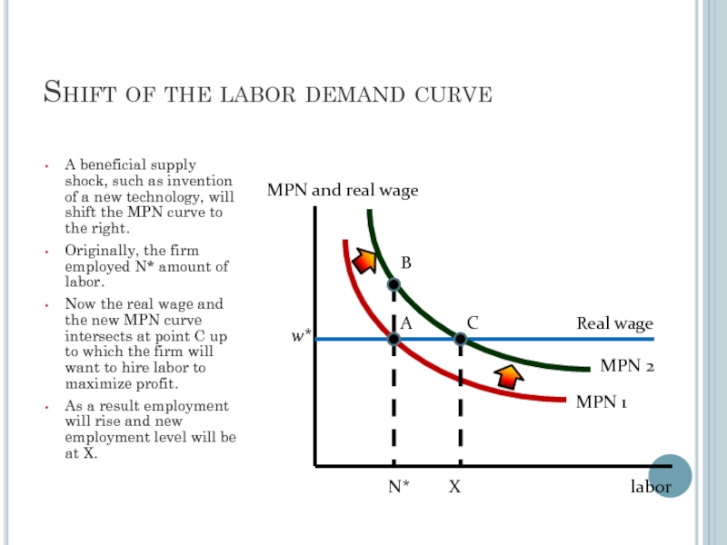
A beneficial supply shock, such as
Originally, the firm employed N* amount of labor.
Now the real wage and the new MPN curve intersects at point C up to which the firm will want to hire labor to maximize profit.
As a result employment will rise and new employment level will be at X.
w*
N*
MPN and real wage
labor
MPN 1
Real wage
A
C
MPN 2
B
X
Слайд 167Supply of labor
We have seen that firm’s demand for labor depend
However, supply of labor depends on workers’ personal choice to work.
Personal choice about being a part of the labor force generally depends on the following two factors:
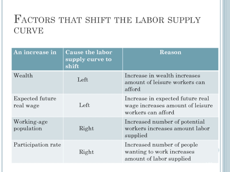
Income-leisure trade-off
Real wage
Слайд 168Labor supply curve
Labor supply curve looks the same as the supply
Usually, we assume that a higher real wage will increase labor supply.
Labor supply curve will not shift because of a change in the wage.
Any factor that changes the amount of labor supply at a given wage rate will shift the labor supply curve.
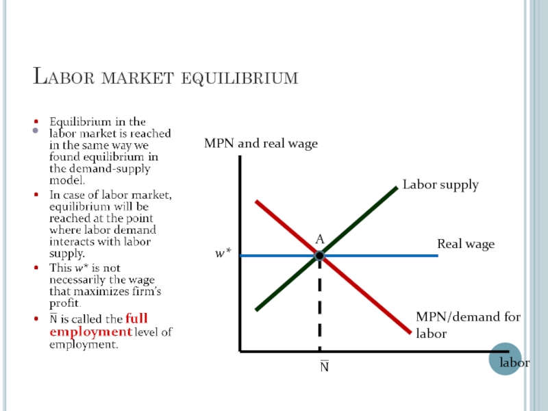
Слайд 170Labor market equilibrium
w*
MPN and real wage
labor
MPN/demand for labor
Real wage
A
Labor supply
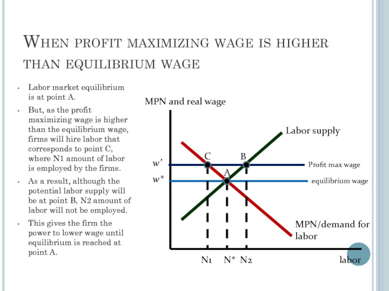
Слайд 171When profit maximizing wage is higher than equilibrium wage
Labor market equilibrium
But, as the profit maximizing wage is higher than the equilibrium wage, firms will hire labor that corresponds to point C, where N1 amount of labor is employed by the firms.
As a result, although the potential labor supply will be at point B, N2 amount of labor will not be employed.
This gives the firm the power to lower wage until equilibrium is reached at point A.
w*
N*
MPN and real wage
labor
MPN/demand for labor
equilibrium wage
A
Profit max wage
w’
C
B
N2
N1
Labor supply
Слайд 172Effects of adverse supply shock
W2
N2
real wage
labor
ND 1
B
N1
ND2
A
W1
NS
1. A temporary adverse supply
2. Employment falls
2. Real wage falls
Слайд 173What if all workers are not alike?
We assumed that all workers
However, if workers have different skill level then supply shocks will not affect all workers in the same way.
Example: if a production process introduces computer based production, then workers who can operate computers will cope with the new process quickly. On the other hand, workers who cannot operate computers will find it difficult to cope with the process. This will create difference in the marginal productivity level of these two groups of workers. Most likely, the workers who can use computers will get higher wage at cost of those who cannot.
Therefore, whether a shock will be considered beneficial or adverse depends on the skill/education level of the workers.
Слайд 174Unemployment: the untold story of full-employment
Full-employment level implies that all the
All workers in real life do not find jobs even if they want to. When workers are unemployed for a long time the sum of all such workers constitute “structural unemployment”.
If workers are unemployed for a brief period (for example: the brief period in which they search for a suitable job) we call it “frictional unemployment”.
The rate of unemployment that prevails when output and unemployment rate the full-employment level, we call it natural rate of unemployment.
The difference between actual unemployment rate and natural unemployment rate is called cyclical unemployment.
If workers are not willing to work, this will not constitute unemployment. We shall consider these workers as out of work force.
Слайд 176GDP Per Capita / GDP PPP (purchasing parity power)
GDP per
The per capita GDP is especially useful when comparing one country to another, because it shows the relative performance of the countries. A rise in per capita GDP signals growth in the economy and tends to reflect an increase in productivity.
Слайд 177Why do we need GDP per capita?
sometimes used as an indicator
NB: A standard of living is the level of wealth, comfort, material goods and necessities available to a certain socioeconomic class or a certain geographic area. The standard of living includes factors such as income, gross domestic product, national economic growth, economic and political stability, political and religious freedom, environmental quality, climate, and safety. The standard of living is closely related to quality of life.
Слайд 179Why do we need GDP per capita?
can also be used to
Methodology: Productivity is calculated by dividing each country's GDP by the average number of hours worked annually by all employed citizens. Hours worked include full-time and part-time workers, excluding holidays and vacation time.
Слайд 180The most productive countries (2015)
NB: Working longer hours doesn't necessarily result
Слайд 182Labour productivity
Labour productivity is defined as real gross domestic product (GDP)
This captures the use of labour inputs better than just output per employee, with labour input defined as total hours worked by all persons involved.
The data are derived as average hours worked multiplied by the corresponding and consistent measure of employment for each particular country. Forecast is based on an assessment of the economic climate in individual countries and the world economy, using a combination of model-based analyses and expert judgement. This indicator is measured as an index with 2010=1.
Слайд 184Labour productivity and utilization
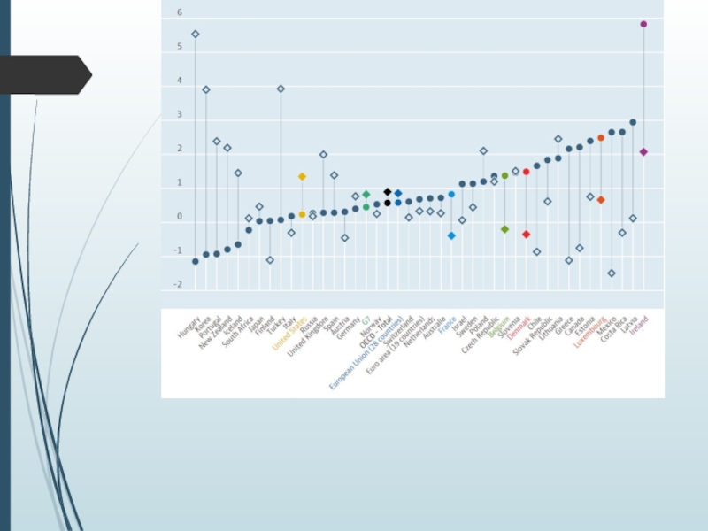
Labour productivity growth is a key dimension of
Слайд 186Multifactor productivity
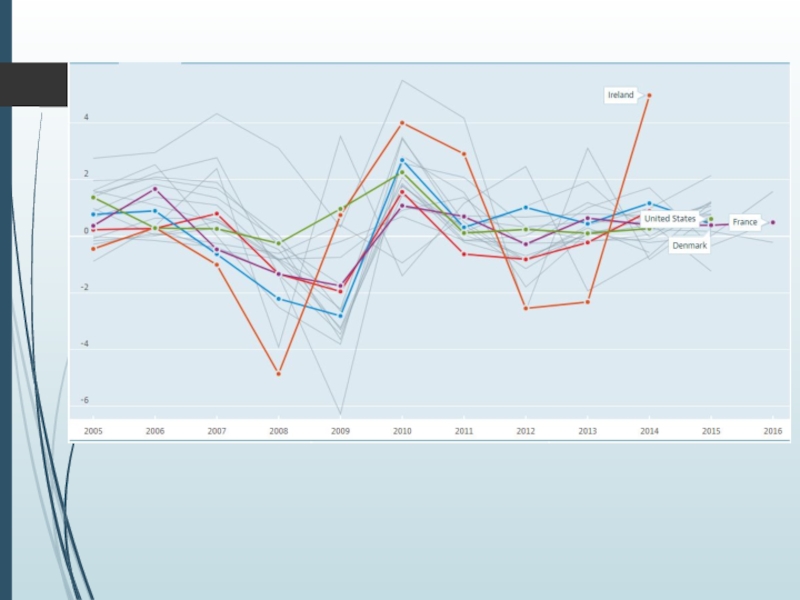
Multifactor productivity (MFP) reflects the overall efficiency with which labour
Growth in MFP is measured as a residual, i.e. that part of GDP growth that cannot be explained by changes in labour and capital inputs. In simple terms therefore, if labour and capital inputs remained unchanged between two periods, any changes in output would reflect changes in MFP. This indicator is measured as an index and in annual growth rates.
Слайд 188What Is Purchasing Power Parity?
Macroeconomic analysis relies on several different metrics
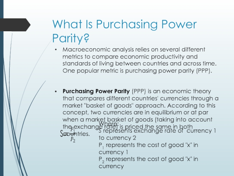
Purchasing Power Parity (PPP) is an economic theory that compares different countries' currencies through a market "basket of goods" approach. According to this concept, two currencies are in equilibrium or at par when a market basket of goods (taking into account the exchange rate) is priced the same in both countries.
Where:
S represents exchange rate of currency 1 to currency 2
P1 represents the cost of good "x" in currency 1
P2 represents the cost of good "x" in currency
Слайд 189PPP calculation
Problem: To make a comparison of prices across countries that
Solution: To facilitate this, the International Comparisons Program (ICP) (established in 1968 by the University of Pennsylvania and UN). Purchasing power parities generated by the ICP are based on a worldwide price survey that compares the prices of hundreds of various goods. This data, in turn, helps international macroeconomists come up with estimates of global productivity and growth.
Correction & Updating: Every three years, the World Bank constructs and releases a report that compares various countries in terms of PPP and U.S. dollars.
Usage: Both the International Monetary Fund (IMF) and the Organization for Economic Cooperation and Development (OECD) use weights based on PPP metrics to make predictions and recommend economic policy.
These actions often impact financial markets in the short run. Some forex traders also use PPP to find potentially overvalued or undervalued currencies. Investors who hold stock or bonds of foreign companies may survey PPP figures to predict the impact of exchange-rate fluctuations on a country's economy.
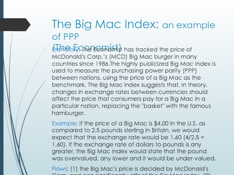
Слайд 190The Big Mac Index: an example of PPP
(The Economist)
Prehistory: The Economist
Example: if the price of a Big Mac is $4.00 in the U.S. as compared to 2.5 pounds sterling in Britain, we would expect that the exchange rate would be 1.60 (4/2.5 = 1.60). If the exchange rate of dollars to pounds is any greater, the Big Mac Index would state that the pound was overvalued, any lower and it would be under-valued.
Flaws: (1) the Big Mac's price is decided by McDonald's Corp. and can significantly affect the Big Mac index. (2) the Big Mac differs across the world in size, ingredients, and availability.
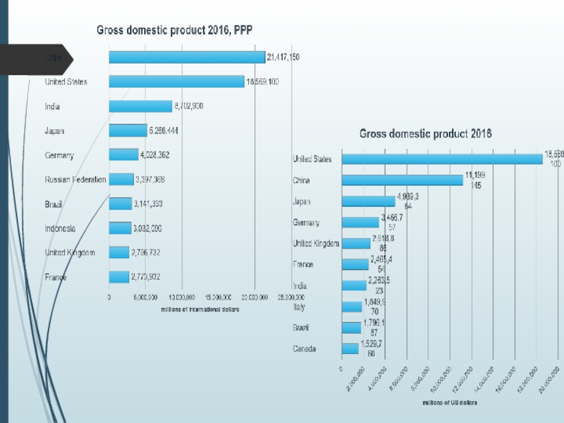
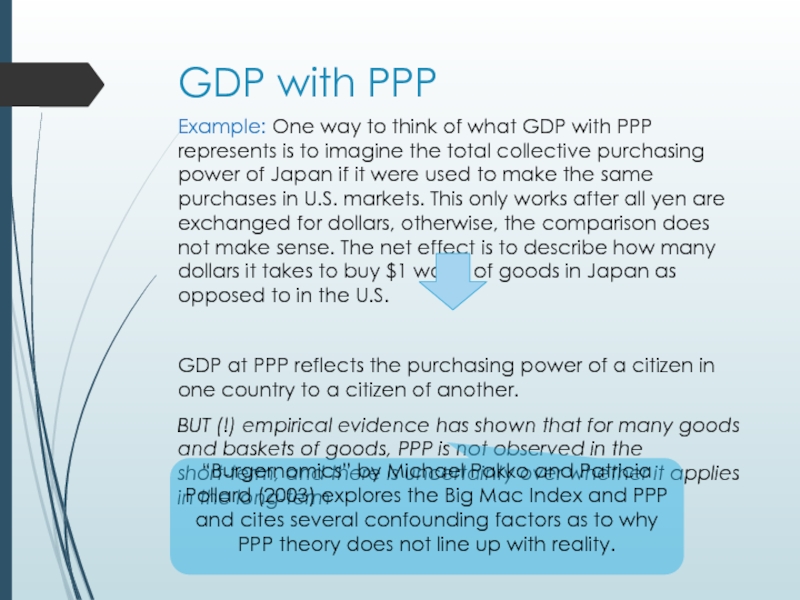
Слайд 192GDP with PPP
Example: One way to think of what GDP with
GDP at PPP reflects the purchasing power of a citizen in one country to a citizen of another.
BUT (!) empirical evidence has shown that for many goods and baskets of goods, PPP is not observed in the short-term, and there is uncertainty over whether it applies in the long-term
“Burgernomics” by Michael Pakko and Patricia Pollard (2003) explores the Big Mac Index and PPP and cites several confounding factors as to why PPP theory does not line up with reality.
Слайд 193Transport Costs: Goods that are not available locally will need to
Taxes: When government sales taxes, such as value-added tax (VAT), are high in one country relative to another, this means goods will sell at a relatively higher price in the high-tax country.
Government Intervention: Import tariffs add to the price of imported goods. Where these are used to restrict supply, demand rises, causing the price of the goods to rise as well. In countries where the same good is unrestricted and abundant, its price will be lower. Governments that restrict exports will see a good's price rise in importing countries facing a shortage, and fall in exporting countries where its supply is increasing.
Non-Traded Services: those costs are unlikely to be at parity internationally. These costs can include the cost of the storefront, and other expenses such as insurance, heating and the cost of labor.
Market Competition: Goods might be deliberately priced higher in a country because the company has a competitive advantage over other sellers, either because it has a monopoly or is part of a cartel of companies that manipulate prices. The company's sought-after brand might allow it to sell at a premium price as well. Conversely, it might take years of offering goods at a reduced price to establish a brand and add a premium, especially if there are cultural or political hurdles to overcome.
Слайд 195From the 10 years of military dictatorship between 1948-1958 to the
But despite these challenges throughout its history, no one has ever denied Venezuela’s economic potential. After the discovery of oil in the early 20th century, the nation quickly built its economy on back of black gold – and even today, Venezuela leads the world in proven oil reserves with 300 billion barrels.
Слайд 196By 1950, as the rest of the world was struggling to
Unfortunately for Venezuela, this wealth wouldn’t last – and an over-reliance on oil would soon decimate the economy in unexpected ways.
Слайд 197The Downfall of Venezuela’s Economy
From 1950 to the early 1980s, the
By 1982, Venezuela was still the richest major economy in Latin America. The country used its vast oil wealth to pay for social programs, including health care, education, transport, and food subsidies. Workers in Venezuela were among the highest paid in the region.
However, from there things went quickly downhill. In the mid-1980s, an oil glut and a free-falling oil price ended up decimating the Venezuelan economy, which was unable to diversify away from energy.
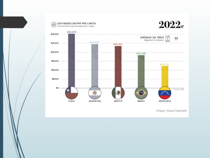
Today, Venezuela has one of the poorest major economies in Latin America – and as the current crisis rides itself out, the IMF foresees it getting far worse. By 2022, the organization predicts Venezuela’s GDP per capita (PPP) will be just $12,210, which would be a massive economic setback – the Venezuelan economy would be even poorer than it was many years before the Chávez era started.
Слайд 199Although oil revenues are tempting to rely on to maintain social
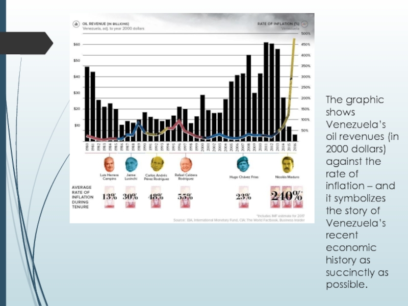
After the oil glut in the 1980s, Venezuela’s oil revenues dropped significantly. It was then that Venezuela had its first bout with inflation, where rates peaked in 1989 (84.5% inflation) and later in 1996 (99.9% inflation). Without sufficient money coming in, the country had to rely on its printing presses in an attempt to maintain living standards
In 1998, Hugo Chávez was elected with the promise that Venezuela could reduce poverty and step up living standards by leaning even more heavily on its energy wealth. The recovery of oil prices helped this come true in the 2000s, and Chávez later passed away in office in 2013.
Слайд 200The graphic shows Venezuela’s oil revenues (in 2000 dollars) against the
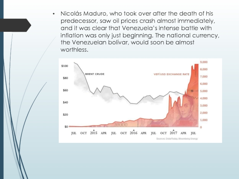
Слайд 201Nicolás Maduro, who took over after the death of his predecessor,
Слайд 202The details of today’s crisis and intense hyperinflation are widely shared.
The country has massive shortages of food, electricity, and other essential goods, and violence is escalating in Caracas. More recently, the government is attempting to tighten its grip around power, and mismanagement of the economy has led to people starving on the streets. People are calling the situation a humanitarian crisis, which is extremely disheartening to see in what was once one of the richest countries on the planet.
And while the current condition of Venezuela is a tragedy in itself, the country’s inability to live up to its true economic potential is nearly just as devastating.
Слайд 204Consumption
Consumption can be defined in different ways, but is usually best
Every time you purchase food at the drive-thru or pull out your debit or credit card or cash to buy something, you are adding to consumption.
Consumption is one of the biggest concepts in economics and is extremely important because it helps determine the growth and success of the economy.
Businesses can open up and offer all kinds of great products, but if we don't purchase or consume their products, they won't stay in business very long
Слайд 205Theories of Consumption
Keynes mentioned several subjective and objective factors which determine
Since Keynes lays stress on the absolute size of income as a determinant of consumption, his theory of consumption is also known as absolute income theory.
Keynes put forward a psychological law of consumption, according to which, as income increases consumption increases but not by as much as the increase in income. In other words, marginal propensity to consume is less than one.
Слайд 206S. Kuznets vision
Contrary to Keynes’s proposition that proportion of income
How the average propensity to consume has remained stable despite the substantial increase in income has been a great puzzle in consumption theory for a long time.
Слайд 208Relative Income Theory of Consumption (J.S. Duesenberry)
Assumptions:
the determinant of consumption
the consumption of a person does not depend on his current income but on certain previously reached income level
because his relative income has remained the same the individual will spend the same proportion of his income on consumption as he was doing before the absolute increase in his income. That is, his average propensity to consume (APC) will remain the same despite the increase in his absolute income.
Слайд 209Demonstration Effect: individuals or households try to imitate or copy the
if incomes of all families increase in the same proportion, distribution of relative incomes would remain unchanged and therefore the proportion of consumption expenditure to income which depends on relative income will remain constant.
family with a given income would devote more of his income to consumption if it is living in a community in which that income is regarded as relatively low because of the working of demonstration effect.
Слайд 210Ratchet Effect - when income of individuals or households falls, their
this is partly due to the demonstration effect. People do not want to show to their neighbours that they no longer afford to maintain their high standard of living.
partly due to the fact that they become accustomed to their previous higher level of consumption and it is quite hard and difficult to reduce their consumption expenditure when their income has fallen. They maintain their earlier consumption level by reducing their savings. Therefore, the fall in their income, as during the period of recession or depression, does not result in decrease in consumption expenditure very much as one would conclude from family budget studies.
Слайд 211Life Cycle Theory of Consumption ( Albert Ando & Franco Modigliani)
Idea: the consumption in any
Assumptions:
to plan a pattern of consumption expenditure based on expected income in their entire lifetime
individual maintains a more or less constant or slightly increasing level of consumption
his level of consumption is limited by his expectations of lifetime income
Слайд 212A typical individual in this theory in his early years of
It is in his main working years of his lifetime that he consumes less than the income he earns and therefore makes net positive savings. He invests these savings in assets, that is, accumulates wealth which he consumes in the future years. In his lifetime after retirement he again dissaves, that is, consumes more than his income in these later years of his life but is able to maintain or even slightly increase his consumption in the lifetime after retirement.
Слайд 213Shortcomings:
criticized the assumption of life cycle hypothesis that in making consumption
theory fails to recognize the importance of liquidity constraints in determining the response of consumption to income. According to critics, even if a household has a concrete vision of future income, the opportunities to borrow from the capital markets for quite a long period on the basis of expected future income are very little.
Слайд 214Permanent Income Theory of Consumption (Milton Friedman)
Assumptions:
consumption is determined by
an individual would prefer a smooth consumption flow per day rather than plenty of consumption today and little consumption tomorrow. Thus consumption in one day is not determined by income received on that particular day.
permanent income or expected long-term average income is earned from both “human and non-human wealth”
Слайд 215Relationship between Consumption and Permanent Income: Cp = k(i,w,u) ×Yp
Cp –
Yp – permanent income
k - the proportion of permanent income that is consumed
Rate of interest (i): at a higher rate of interest the people would tend to save more and their consumption expenditure will decrease.
The proportion of non-human wealth to human wealth (w): the greater the amount of wealth or assets held by an individual, the greater would be its propensity to consume and vice-versa
Desire to add to one’s wealth (u): households’ preference for immediate consumption as against the desire to add to the stock of wealth or assets also determines the proportion of permanent income to be devoted to consumption
Слайд 216In addition to permanent income (Yp), the individual’s income may contain
When income of an individual increases in the current year as compared to the last year, the permanent income will be less than the current year’s income. This is because individual is not sure whether the increase in income will persist in the future and therefore does not immediately revise his estimate of permanent income by the full amount of the increase in his income in the current year
Слайд 217Conclusions:
Permanent income hypothesis is similar to life cycle hypothesis and
Permanent income hypothesis is also consistent with the evidence from the cross-sectional budget studies that high income families have low average propensity to consume than that of low- income families. A sample of high income families at a given time is likely to contain a relatively larger number of families who are having positive transitory increase in incomes.
laying stress on changes in rate of interest and the wealth or assets held by the people and desire to add to one’s wealth as important determinants of consumption and savings, Friedman’s permanent income hypothesis has made an important contribution to the theory of consumption and saving.
Слайд 218Real income vs. nominal income
The term 'real' that is used in
Слайд 219Savings
Savings, according to Keynesian economics, consists of the amount left over when
Saving involves income that is not consumed
Savings can be turned into further increased income through investing in different investment vehicles.
Saving is often confused with investing, but they are not the same.
Although most people think of purchases of stocks and BONDS as investments, economists use the term “INVESTMENT” to mean additions to the real stock of capital: plants, factories, equipment, and so on
Слайд 221Investments
Definition: Money committed or property acquired for future income.
“INVESTMENT” to mean
An investment is an asset or item that is purchased with the hope that it will generate income or will appreciate in the future. In an economic sense, an investment is the purchase of goods that are not consumed today but are used in the future to create wealth. In finance, an investment is a monetary asset purchased with the idea that the asset will provide income in the future or will be sold at a higher price for a profit.
Слайд 222Leverage Firms (Companies), are the best place to invest, because it’s
Always invest in that firm or thing whose rate of return or profitability in future is high
Fixed Investment - is spending on new capital machinery and plant, construction, housing, vehicles, etc.
Working Capital - is spending on stocks/ inventories of finished goods and raw materials. The accumulation of stocks by firms, whether voluntary or involuntary, is counted as investment
Слайд 224Final Conclusions
Consumed is what you buy or ability to pay.
High consumption
If consumption is not high then product will failed.
Saving is what you have after all your expenses.
Saving is not what you invest.
Investment is for the future profits.
Investment made when the earning per share of the company is high.
Слайд 226GDP = is the monetary value of all the finished goods
Includes all domestic production in a boarders
Monetary measurement of value
To avoid multiple counting – must include ONLY new production (sold to consumers)
Does NOT include:
intermediate goods (ex: tires for new auto)
public transfer payments (welfare payment)
private transfer payments (cash gifts)
stock market transactions (stocks & bonds)
secondhand sales (used books, cars, homes)
Слайд 227Approaches to calculate GDP
Expenditure & Income Methods
Expenditure Method – count all
GDPExpenditure =C + I + G + NX
Consumption
Investment
Government purchases of goods and services
Net eXports
Слайд 236Expenditure approach for 1 product economy
Roaster
Wages $15,000
Taxes $5,000
Revenue $35,000
beans sold to public
beans sold to coffee bar $25,000
Coffee bar
Wages $10,000
Taxes $2,000
Beans bought from roaster $25,000
Revenue from coffee sold to public $40,000
Note: Beans sold to coffee bar are intermediate goods since they are used in the production of coffee sold to the public (final good).
Total expenditure = Consumption Expenditures = Beans purchased by public + Coffee purchased by public = $10,000 + $40,000 = $50,000 final goods.
Слайд 237Expenditure approach for 1 product economy
Winegrower
Wages $20,000
Taxes $7,000
Revenue $50,000
sold to public
sold to wine-maker $30,000
Wine-maker
Wages $18,000
Taxes $8,000
Grapes from winegrower $30,000
Revenue from wine sold to public $40,000
Total expenditure = Consumption Expenditures = Grapes purchased by public + Wine purchased by public = 20 000 + 40 000 = 60 000 final goods.
Слайд 238Product approach
GDP is the sum of the value added created in
Value added is sales minus materials, intermediate inputs and energy costs.
The value of a final good is equal to the value added at each stage of production.
Expenditure method = Production Method
Слайд 239Product approach for 1 product economy
Roaster
Wages $15,000
Taxes $5,000
Revenue $35,000
beans sold to public
beans sold to coffee bar $25,000
Coffee bar
Wages $10,000
Taxes $2,000
Beans bought from roaster $25,000
Revenue from coffee sold to public $40,000
Value Added – revenue earned by selling products minus the amount paid for intermediate goods
Intermediate goods - goods that are used for the production of other goods (in the current year)
Roaster value added = $35,000 in revenue - $0 spent on intermediate goods = $35,000
Coffeebar value added = $40,000 in revenue - $25,000 spent on intermediate goods (beans) = $15,000
Total value added = $50,000
Слайд 240Expenditure approach for 1 product economy
Winegrower
Wages $20,000
Taxes $7,000
Revenue $50,000
sold to public
sold to wine-maker $30,000
Wine-maker
Wages $18,000
Taxes $8,000
Grapes from winegrower $30,000
Revenue from wine sold to public $40,000
Winegrower value added = 50 000 in revenue – 0 spent on intermediate goods = 50 000
Wine-maker value added = 40 000 in revenue – 30 000 spent on intermediate goods (beans) = 10 000
Total value added = 50 000 + 10 000 = 60 000
Слайд 241Income method
Income Method – count all earnings received by those who
Workers, owners of property, interest earned on savings, profit earned by business owners (proprietors, partners & corporation stockholders)
Requires some accounting adjustments => Expenditures = Income (must balance)
National income => all citizens supplied resources (here & abroad)
National Income + statistical discrepancy = Net National Product
Слайд 242Consumption (C)
Investment (I)
Government purchases (G)
Exports (X)
Imports (M)
Taxes (T)
Saving (S)
(I
Слайд 243Consumption
+
Investment
+
Government
+
Net Export
Wages
+
Profits
+
Rents
+
Interest
Depreciation (CCA)
Indirect business taxes (IBT)
GDP in market prices
National income
Expenditure approach
Income
W - employee compensation (wages)
P - profits received by proprietors & corporation owners (income taxes, dividends, & undistributed profits (retained earnings)
R - rent received for use of property
I - Interest received for use of money
Compensation of Fixed Capital = Depreciation (costs of capital over its lifetime)
Sales, excise, property, customs duties, license fees, etc
Слайд 244
NFIA = Factor income earned from abroad by residents - Factor
Слайд 246Income approach for 1 product economy
Roaster
Wages $15,000
Taxes $5,000
Revenue $35,000
beans sold to public
beans sold to coffee bar $25,000
Coffee bar
Wages $10,000
Taxes $2,000
Beans bought from roaster $25,000
Revenue from coffee sold to public $40,000
Note: profit = revenue - expenses
Total wages: $15,000 + $10,000 = $25,000
Total taxes: $5,000 + $2,000 = $7,000
Roaster profit = Revenue - Expenses = $35,000 - ($15,000 in wages + $5,000 in taxes) = $15,000.
Coffeebar profit = Revenue - Expenses = $40,000 - ($10,000 in wages + $2,000 in taxes + $25,000 in beans) = $3,000
Total profit = $15,000 + $3,000 = $18,000.
Total income = Total Wages + Total Taxes + Total Profits = $25,000 + $7,000 +$18,000 = $50,000
Слайд 247Income approach for 1 product economy
Winegrower
Wages $20,000
Taxes $7,000
Revenue $50,000
sold to public
sold to wine-maker $30,000
Wine-maker
Wages $18,000
Taxes $8,000
Grapes from winegrower $30,000
Revenue from wine sold to public $40,000
Total wages = 20 000+18 000 = 38 000
Total taxes = 7 000+8 000 = 15 000
Profit (winegrower) = 50 000 - (20 000+7 000) = 23 000
Profit (wine-maker) = 40 000 - (18 000+8 000+30 000) = -16 000
Total revenue = 23 000 – 16 000 = 7 000
Total income = 38 000+150 00+7 000 = 60 000
Слайд 249The first account displays the expenditure and income approaches to measuring
Слайд 250GDP (BEA commentaries)
The entries on the right side of account 1
The left (income) side – the sum of all the incomes earned and costs incurred in production.
Specifically, the left side shows GDI as the sum of the income earned by labor, governments and entrepreneurs and the consumption of fixed capital.
In theory, GDI should be equal to GDP. In practice, differences in the source data used to estimate the two measures result in a “statistical discrepancy,” which, in the NIPAs ( national income and product accounts), is calculated as GDP less GDI.
Because the source data used to develop the product-side estimates of the account are based on more comprehensive surveys and censuses, BEA considers them more reliable. Therefore, the statistical discrepancy appears as a component on the income side of the account to equate GDI with GDP.
Слайд 252GDP – Nominal vs. Real
Nominal = current year prices
Real = prices
Nominal > Real (in the most cases)
Nominal GDP is used when comparing different quarters of output within the same year. When comparing the GDP of two or more years, real GDP is used because, by removing the effects of inflation, the comparison of the different years focuses solely on volume.
Слайд 255Example
Nominal GDP =Pcheese∗QCheese+Pcheese∗QCheese
Nominal GDP =Pcheese∗Qcheese+Pwine∗Qwine
Nominal GDP2010 = 5*2+10*4=50
Nominal GDP2011=12*3+17*3=87
Nominal GDP2012=12*4+20*3=108
Real
Real GDP2010 = 5*2+10*4=50
Real GDP2011=5*3+10*3=45
Real GDP2012=5*4+10*3=50
Real GDP grow = (Real GDP 2011-Real GDP 2010)/Real GDP2010
Real GDP grow2011-2010 = (45-50)/50= -0.1
Real GDP grow2011-2012 = (50-45)/50= 0.1
Nominal GDP grow2011-2010 = (87-50)/50= 0.74
Nominal GDP grow2011-2012 = (108-87)/87= 0.24
Based year
Слайд 256where
GDPt is the level of activity in the later period;
GDP0 is the level
m is the periodicity of the data (for example, 1 for annual data, 4 for quarterly data, or 12 for monthly data); and
n is the number of periods between the earlier period and the later period(that is t-0).
Слайд 257Deflator GDP
GDP deflator is an index of the price level relative
It is the cost of purchasing the goods that represent GDP relative to the cost of purchasing the exact same goods if they had been sold at the prices prevailing in the base year
Consumer Price Index
The CPI is a measure that examines the weighted average of prices of a basket of consumer goods and services
Price index in the base year is always 100
Слайд 258GDP deflator =
Nominal GDP
Real GDP
× 100%
Total amount of money on GDP
Corrects the value of Nominal GDP for inflation
Слайд 259What is the relationship between GDP deflator & CPI?
Both GDP
GDP deflator measures price level but will focus more on all new, domestically produced, final goods and services in an economy
CPI is the measure of changes in the price level of consumer goods purchased by households over time.
CPI uses a fixed basket to compare prices in determining inflation progress. GDP deflator uses the price of the currently produced product relative to the price from the base year.
Слайд 261Example
The value of this market basket in the base year :
5
The value of the market basket in the year 2012 :
12 × 1+20 × 2=52
CPI2012= (52/25) × 100= 208
Deflator GDP2010 = (Nominal GDP2010/Real GDP2010 ) × 100=(50/50) ×100=100
Deflator GDP2012=(108/50) ×100=216
Inflation=[(Def GDP2012-Def GDP2010)/Def GDP 2010] ×100=[(216-100)/100] ×100=216
To convert a nominal value to a real value:
So a Television that cost $100 in 2012 would cost $48 ([100/208] × 100=48) (CPI) or $46.3 ([100/216] × 100=46.3) (Deflator GDP) in 2010
Real GDP 2012 in 2010 dollars =50×(100/216)=23.14
Слайд 262Define Inflation as the growth rate of prices.
The greek letter π
Inflation means that prices are growing
Disinflation means that inflation is slowing down but still positive
Deflation means that inflation is negative and prices are actually dropping.
Inflation
Слайд 264Example
In 1966, Howard Hughes was forced to sell TWA (trans world
The GDP deflator in USA in 1966 was 22.855. The deflator in 2004 was 107.958.
In 2004 dollars this is
Слайд 265Trends and cycles
We observe that real GDP is growing over time
We call the growth path, if the economy were always growing at its average rate, the trend path.
Fluctuations around the trend are called business cycles.
Слайд 266Business Cycle term
As the economy fluctuates around the trend, the economy
When economy is moving from a peak level to trough level, the economy is in a contractionary phase.
When economy is moving from trough to peak, the economy is in an expansionary phase.
When economy is moving from peak to trough the economy is in a contractionary phase
Слайд 267The correlation of business cycles implies that groups of countries are
Слайд 268North American Free Trade Agreement (NAFTA)
It is a piece of regulation
The essence of a free trade measure, NAFTA’s purpose is to encourage economic activity between the three major economic powers of North America.
NAFTA has two supplements: the North American Agreement on Environmental Cooperation (NAAEC) and the North American Agreement on Labor Cooperation (NAALC).
About 1/4 of all U.S. imports (especially crude oil, machinery, gold, vehicles, fresh produce, livestock and processed foods) comes from Canada and Mexico, which are the United States’ second- and third-largest suppliers of imported goods. In addition, about one-third of U.S. exports, particularly machinery, vehicle parts, mineral fuel/oil and plastics are destined for Canada and Mexico.
Слайд 269The global expansion remains relatively steady and synchronized across major economies.
Broadly
The Eurozone is not as far along as the U.S. in the cycle, and it continues to benefit from improving sentiment and credit conditions.
China's activity has rebounded to multiyear highs, but policy tightening and slowing momentum in industrial activity and housing suggest that most of the upside has already occurred.
Overall, the global expansion is on firm ground, but peak activity levels have probably already been reached.
Слайд 270Recession and booms
Business cycle positions are sometimes characterized as booms and
These names have many definitions
a boom occurs roughly when real output is above the trend growth path (detrended output is positive).
A recession occurs roughly when real output is below trend growth.
In the USA, recessions are sometimes defined as 2 consecutive periods of negative growth.
Слайд 272 Business Cycles & Co-movement
Business cycles are fluctuations in the economy
Different sub-categories of GDP tend to co-move with business cycles though to different degree.
Business cycles tend to co-move across countries though not as strongly as within countries.
Слайд 273Business Cycles & Sub-Categories
Expenditure. Consumption and Investment co-move with output. Investment
Production – Production sectors co-move with business cycles. Manufacturing & Construction most volatile. Services least volatile.
Income – Worker Compensation & Capital Income are both pro-cyclical. Capital Income tends to be more volatile.
Слайд 275Corporate Profits
Corporate profits are strongly pro-cyclical and volatile.
When the economy is
Corporate profits fluctuate far more than the economy as a whole
HK Corporate Earnings & the Business Cycle
Слайд 276Using financial market data to predict business cycles
It has been joked
(In fact there does seem to be a moderately strong, positive correlation between cyclical variation in stock prices and business cycles)
In the USA, some financial market indicators have been shown to predict business cycles.
Default Spread : Interest rates on lower rated bonds vs. Interest rates on better rated bonds.
Term Spread: Interest rates on long-term bonds vs. short-term bonds (when this is inverted, recession is likely)
Слайд 277The traditional business cycle frequency is around one to eight years.
Слайд 280Unemployment
Is defined by the International Labor Organization (ILO) as a situation
According to this definition, people who do not look for a job will not be considered unemployed.
Productive population
In the labor force
Not in the labor force
Employed
Unemployed
Слайд 281Unemployment
Labor force
Many people who would like to work but cannot (due
Слайд 282Employment dynamics
Employed labor force
Unemployed
New hire/ recall
Lay off/ quits
Out of the labor
Retiring/ temporarily leaving
Taking a job
Discouraged workers
New entrants willing to work but not yet found one
A discouraged worker is a person who is eligible for employment and is able to work, but is currently unemployed and has not attempted to find employment in the last four weeks.
Слайд 283Example
Who is counted as employed?
On vacation
Ill
Experiencing child care problems
On maternity or
Taking care of some other family or personal obligation
Involved in a labor dispute
Prevented from working by bad weather
Fictional scenarios:
Elena reported to the interviewer that last week she worked 40 hours as a sales manager for a beverage company. Elena is employed.
Steve lost his job when the local plant of an aircraft manufacturing company closed down. Since then, he has been contacting other businesses in town trying to find a job. Steve is unemployed.
Linda is a stay-at-home mother. Last week, she was occupied with her normal household activities. She neither held a job nor looked for a job. Her 80-year-old father who lives with her has not worked or looked for work because of a disability. Linda and her father are not in the labor force.
Слайд 284Example
Garrett is 16 years old, and he has no job from
Lisa spends most of her time taking care of her home and children, but she helps in her husband's computer software business all day Friday and Saturday.
Both Garrett and Lisa are considered employed. They fall into a group called unpaid family workers, which includes any person who worked without pay for 15 hours or more per week in a business or farm operated by a family member with whom they live. Unpaid family workers comprise a small proportion of total employment. Most of the employed are either wage and salary workers (paid employees) or self-employed (working in their own business, profession, or farm).
In addition to estimating the number of employed people, the survey collects information about the job characteristics of the employed. For example, the survey gathers and provides data about workers’ industry and occupation, hours worked, usual earnings, and union membership.
Слайд 286Underemployment
Underemployment is a measure of employment and labor utilization in the
Labor that falls under the underemployment classification includes those workers who are highly skilled but working in low paying jobs, workers who are highly skilled but working in low skill jobs and part-time workers who would prefer to be full time. This is different from unemployment in that the individual is working but is not working at his full capability.
Слайд 287Disguised (hidden) Unemployment
Disguised unemployment exists where part of the labor force
exists frequently in developing countries whose large populations create a surplus in the labor force. It can be characterized by low productivity and frequently accompanies informal labor markets and agricultural labor markets, which can absorb substantial quantities of labor.
can refer to any segment of the population not employed at full capacity, but it is often not counted in official unemployment statistics within the national economy. This can include those working well below their capabilities, those whose positions provide little overall value in terms of productivity, or any group that is not currently looking for work but is able to perform work of value
Слайд 288Alternative Measures
U-1 People who have been unemployed for 15 weeks or
U-2 People who lost their jobs, or whose temporary jobs ended, as a percentage of the labor force.
U-4 Unemployed people, plus discouraged workers, as a percentage of the labor force (plus discouraged workers).
Discouraged workers are those who are available to work and would like a job, but have given up actively looking for one.**
Слайд 289Alternative Measures
U-5 Unemployed people, plus those who are marginally attached to
People who are marginally attached to the labor force include discouraged workers and anyone else who would like a job and has looked for one in the past 12 months, but have given up actively searching. As with U4, the denominator is expanded to include the marginally attached, who are not technically part of the labor force.
Слайд 290Alternative Measures
U-6 Unemployed people, plus people who are marginally attached to
This metric is the Bureau of Labor Statistics (BLS) most comprehensive. In addition to the categories included in U5, it accounts for people who have been forced to settle for part-time work even though they want to work full-time. This category is often referred to as "underemployed," although that label arguably includes full-time workers who are overqualified for their jobs. The denominator for this ratio is the same as in U5.
Слайд 292Tightly regulated labor markets increase structural unemployment.
High social welfare benefits increase
Слайд 293How to solve the problem
There are two ways the government can
There are passive programs, such as unemployment insurance, that help the unemployed make ends meet and stabilize the economy by providing funds that are generally spent immediately. Then there are active programs, such as might help the unemployed meet the skills requirements of available jobs.
Active labor market policies (ALMP). They can be divided into six categories:
Training programs to help workers move from one industry and occupation to another.
Job-search assistance to help match the unemployed with employers.
Employment incentives for employers.
Supported employment to subsidize cost of new hires.
Direct job creation of government spending programs.
Other policies, which can be diverse, including entrepreneurship incentives
Слайд 295Aggregate Demand (AD)
Aggregate demand is the total demand for goods and
is an economic measurement of the sum of all final goods and services produced in an economy, expressed as the total amount of money exchanged for those goods and services.
AD = total spending on goods and services = Real GDP
AD = C+I+G+NX
C - Consumer spending on goods and services
I - Private investment and corporate spending for non-final capital goods (factories, equipment, etc.)
G - Government spending for public goods and social services (infrastructure, Medicare, etc.)
NX = Net exports (exports minus imports)
Real GDP
Wealth effect
Savings and Interest rate effect
Foreign exchange effect
Слайд 296AD shifts
AD = C+I+G+NX
change in consumption (eg cut tax)
Or tax increasing
Shifts in
Investment
Governmental spending
Export
Слайд 297Components of AS
Consumer goods. Private consumer goods and services, such as motor
Capital goods. Capital goods, such as machinery, equipment, and plant, are supplied to other firms.
Public and merit goods. Goods and services produced by private firms for use by central or local government, such as education and healthcare, are also a significant component of aggregate supply.
Traded goods. Goods and services for export, such as chemicals, entertainment, and financial services are also a key component of aggregate supply.
Aggregate supply (AS)
(or total output) is the total supply of goods and services produced within an economy at a given overall price level in a given time period.
Слайд 298Long-run Aggregate supply (LRAS)
Supply = capability to produce
Population growth
Easy to find
More productive (new resources…)
…
War, conflicts …
Слайд 299Sort-run Aggregate Supply (SRAS)
Rising the price – labor pool, work more,
Decreasing price – more leisure time…
Shape
Misperception theory:
Sticky wages (cost/prices) theory
Слайд 300Summirising
Aggregate supply is the total quantity of output firms will produce and
The upward-sloping aggregate supply curve – also known as the short run aggregate supply curve – shows the positive relationship between price level and real GDP in the short run.
The aggregate supply curve slopes up because when the price level for outputs increases while the price level of inputs remains fixed, the opportunity for additional profits encourages more production.
Potential GDP, or full-employment GDP, is the maximum quantity that an economy can produce given full employment of its existing levels of labor, physical capital, technology, and institutions.
Aggregate demand is the amount of total spending on domestic goods and services in an economy.
The downward-sloping aggregate demand curve shows the relationship between the price level for outputs and the quantity of total spending in the economy.
Слайд 301Equilibrium in the aggregate demand/aggregate supply model
At a relatively low price
Real GDP
AD
LRAS
SRAS
E
Conclusions
If equilibrium occurs in the flat range of AS, then economy is not close to potential GDP and will be experiencing unemployment but stable price level. If equilibrium occurs in the steep range of AS, then the economy is close to or at potential GDP and will be experiencing rising price levels or inflationary pressures, but will have a low unemployment rate.
Слайд 302Price level: aggregate demand/aggregate supply
Conclusions: the equilibrium is fairly far from
Слайд 303Example
Bebebe. The imaginary country of Bebebe has the aggregate supply and
Plot an AD/AS diagram from the data above. Identify the equilibrium.
Would you expect unemployment in this economy to be relatively high or low? Would you expect concern about inflation in this economy to be relatively high or low?
Imagine that consumers begin to lose confidence about the state of the economy, so AD becomes lower by 275 at every price level.
Identify the new aggregate equilibrium. How will the shift in AD affect the original output, price level, and employment?
Слайд 304How productivity growth shifts the AS curve
Over time, productivity grows so
A higher level of productivity shifts the SRAS curve to the right because with improved productivity, firms can produce a greater quantity of output at every price level.
Слайд 306Summary
The aggregate demand/aggregate supply model is a model that shows what determines total
Movements of either the aggregate supply or aggregate demand curve in an AD/AS diagram will result in a different equilibrium output and price level.
The aggregate supply curve shifts to the right as productivity increases or the price of key inputs falls, making a combination of lower inflation, higher output, and lower unemployment possible.
The aggregate supply curve shifts to the left as the price of key inputs rises, making a combination of lower output, higher unemployment, and higher inflation possible.
When an economy experiences stagnant growth and high inflation at the same time it is referred to as stagflation.
Слайд 307How do changes by consumers and firms affect AD?
When consumers feel
Consumer and business confidence often reflect macroeconomic realities. For example, confidence is usually high when the economy is growing briskly and low during a recession. However, economic confidence can sometimes rise or fall due to factors that do not have a close connection to the immediate economy, like a risk of war, election results, foreign policy events, or a pessimistic prediction about the future by a prominent public figure.
Слайд 308Government macroeconomic policy choices can shift AD.
Take, for example, government spending–one
Слайд 309During a recession, when unemployment is high and many businesses are
The original equilibrium during the recession is at point E0 relatively far from the full-employment level of output. The tax cut, by increasing consumption, shifts the AD curve to the right. At the new equilibrium E1 real GDP rises and unemployment falls and – because in this diagram the economy has not yet reached its potential or full-employment level of GDP – any rise in the price level remains muted.
Слайд 310Summary
The aggregate demand/aggregate supply model is a model that shows what determines total
The aggregate demand curve shifts to the right as the components of aggregate demand–consumption spending, investment spending, government spending, and spending on exports minus imports–rise. The AD curve will shift back to the left as these components fall.
AD components can change because of different personal choices–like those resulting from consumer or business confidence–or from policy choices like changes in government spending and taxes.
If the AD curve shifts to the right, then the equilibrium quantity of output and the price level will rise. If the AD curve shifts to the left, then the equilibrium quantity of output and the price level will fall.
Whether equilibrium output changes relatively more than the price level or whether the price level changes relatively more than output is determined by where the AD curve intersects with the AS curve.



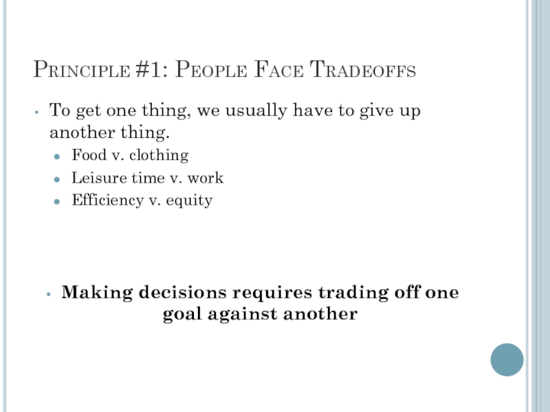

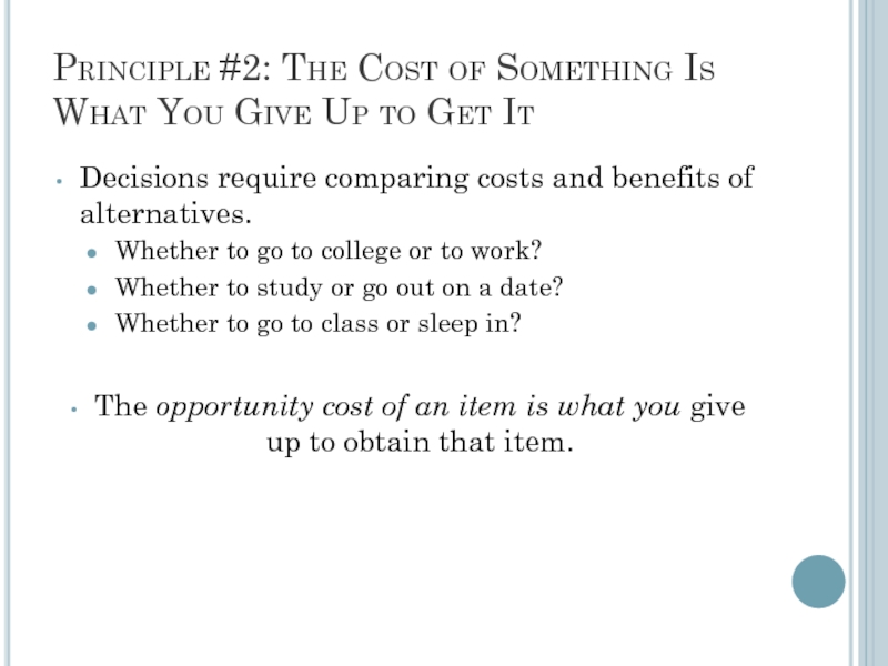

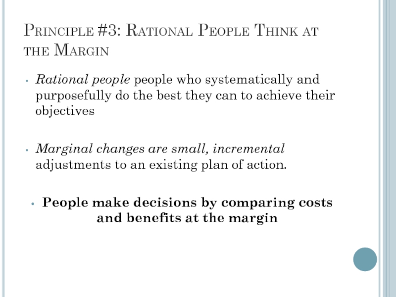
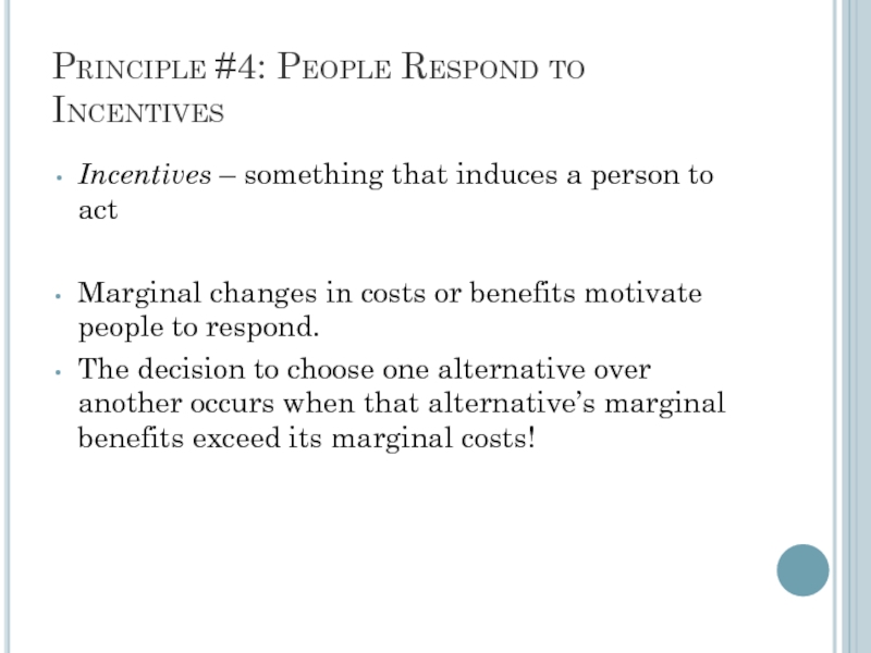
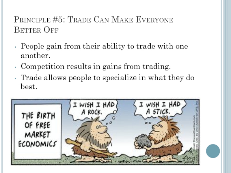







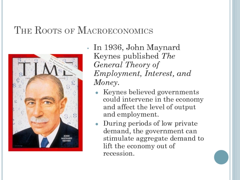
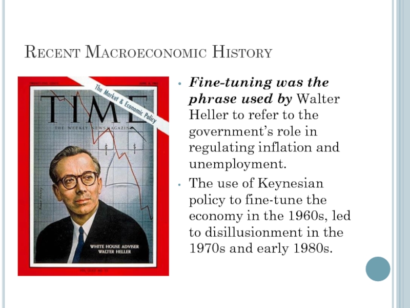

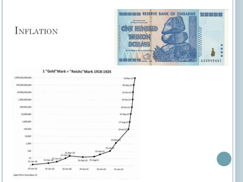

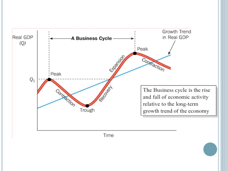
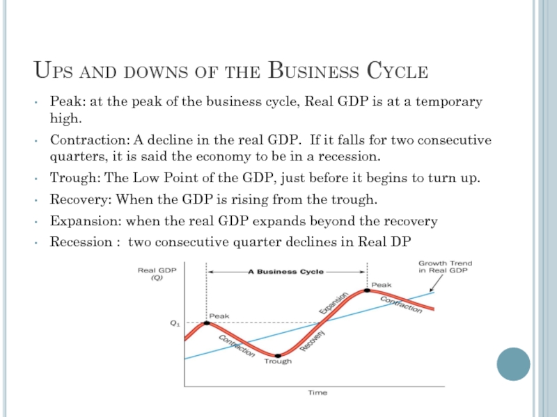

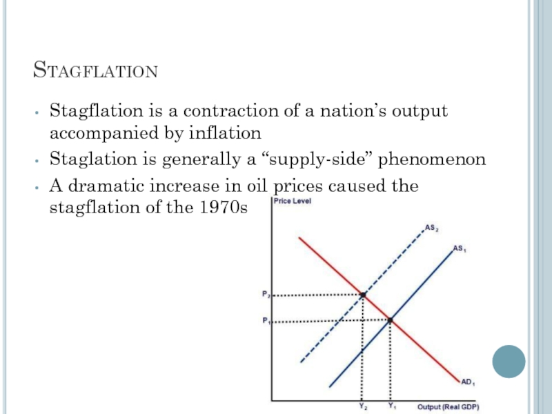


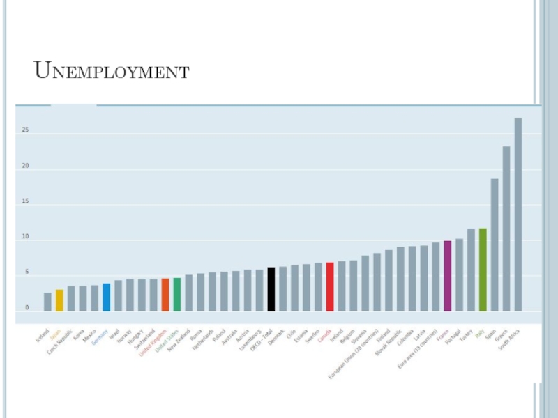
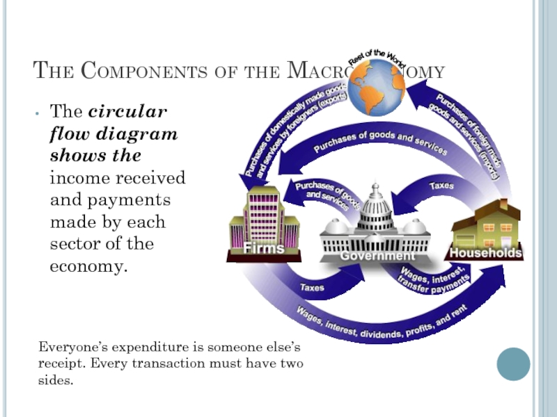
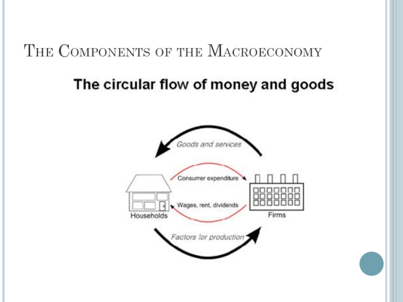
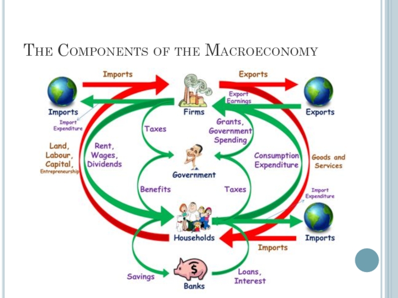

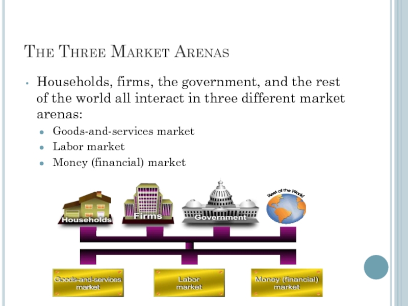

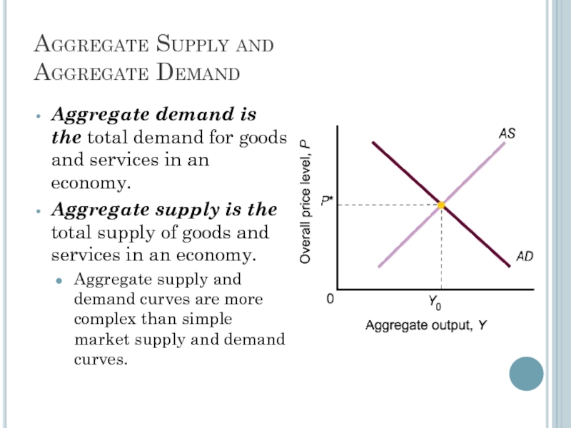
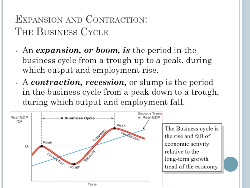
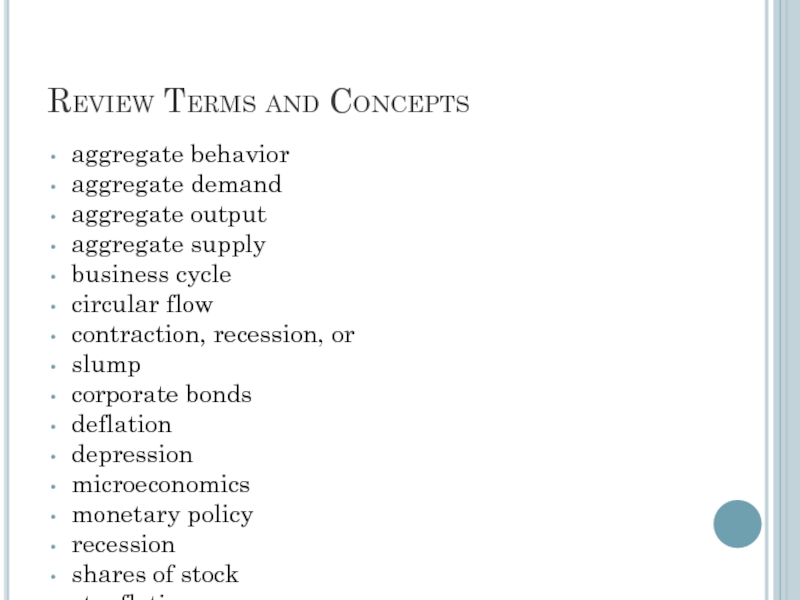


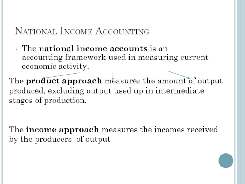
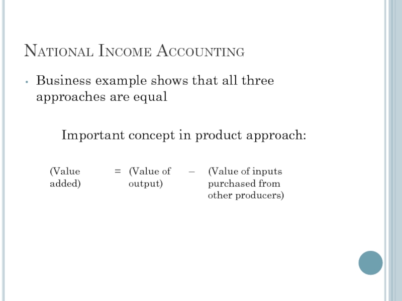
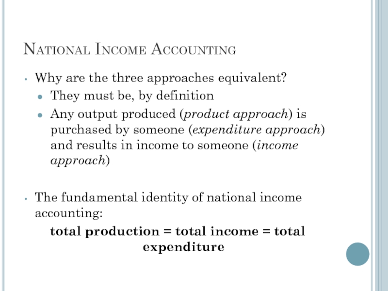
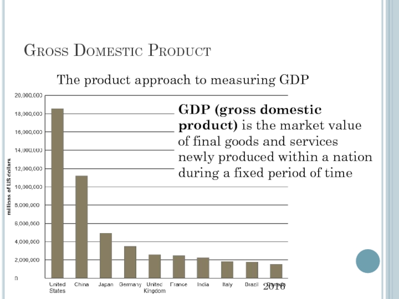
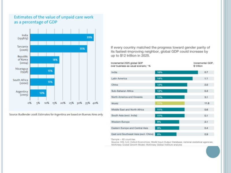
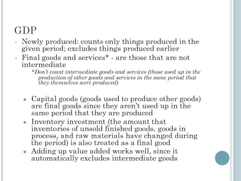
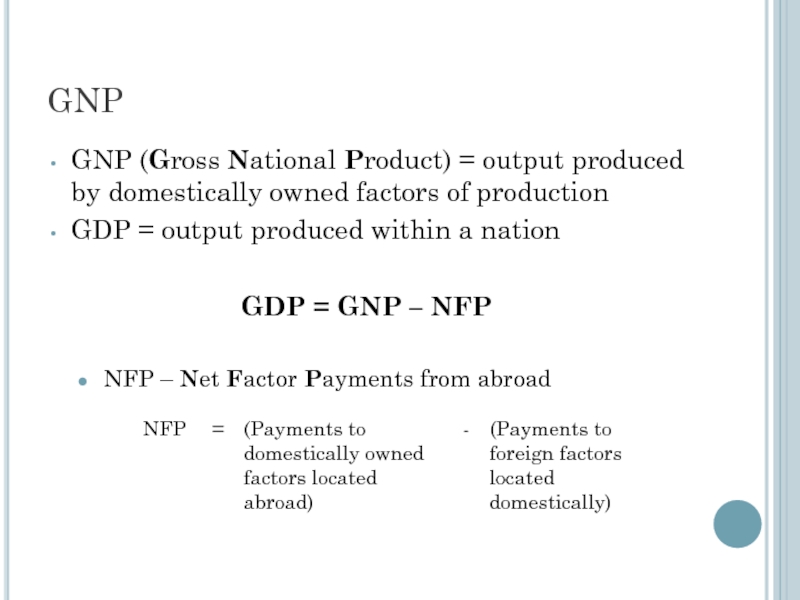


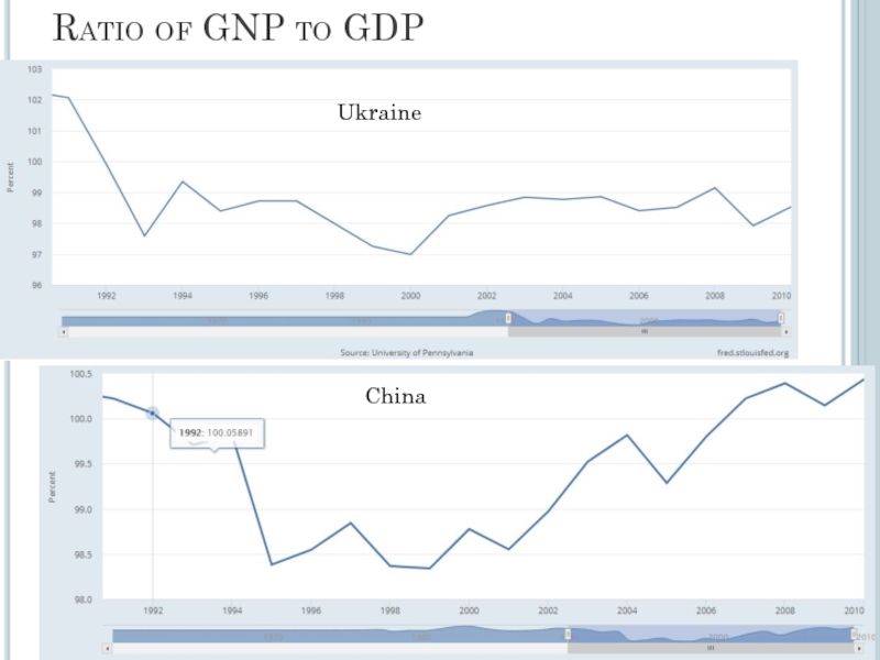
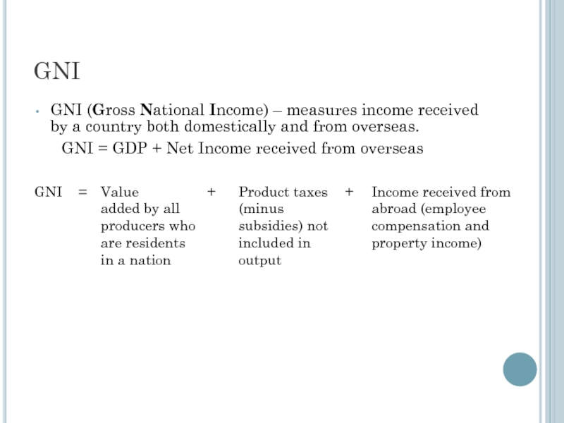
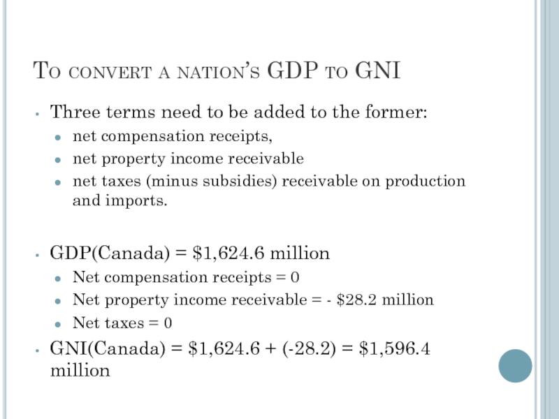

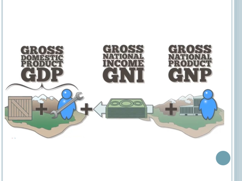

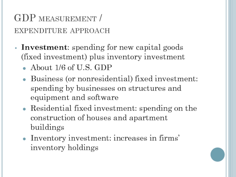
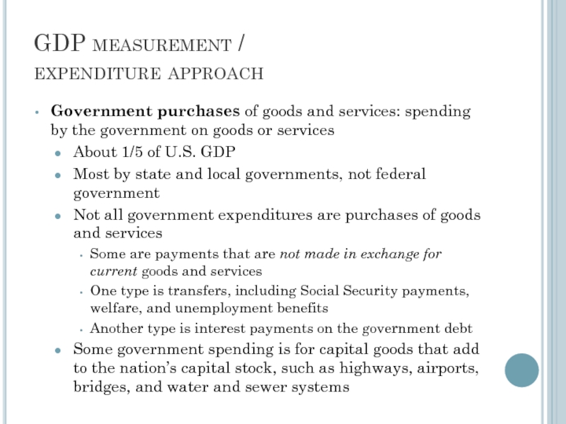

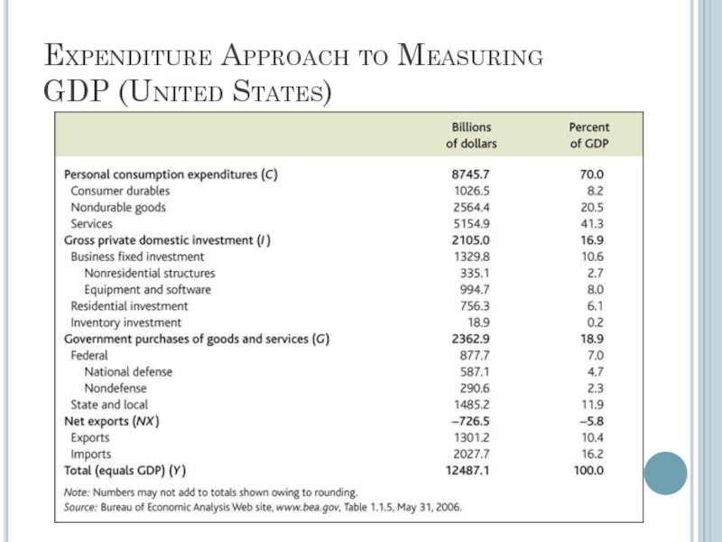
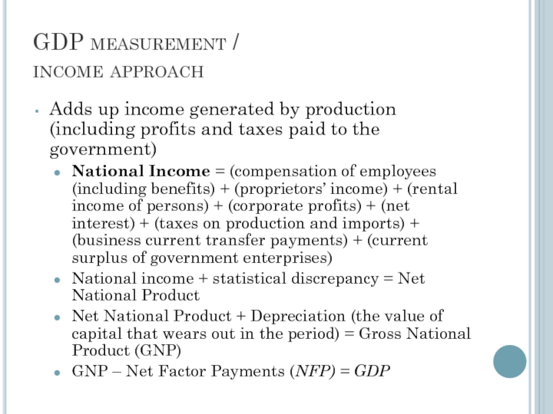
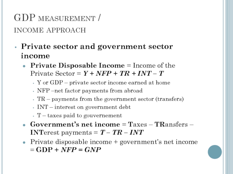

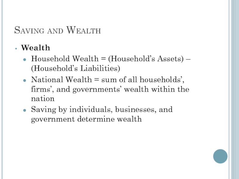
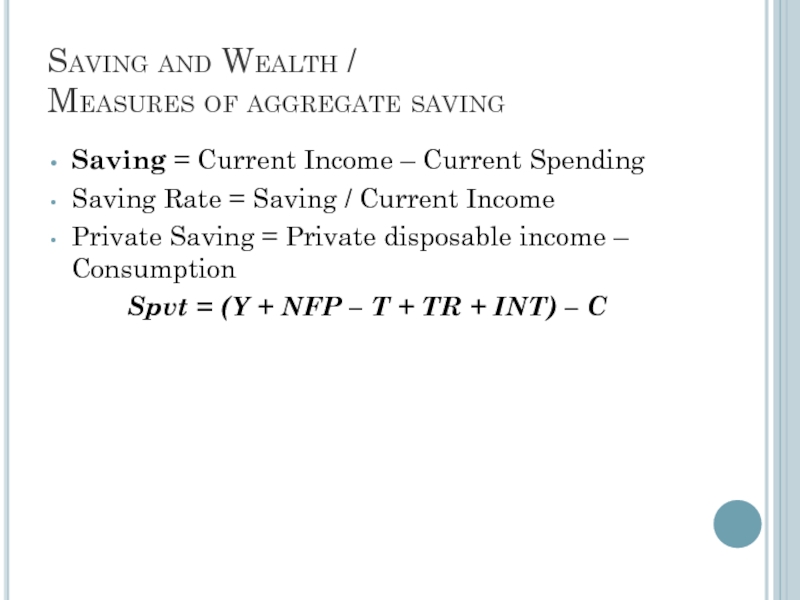
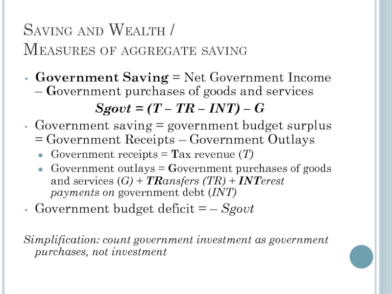


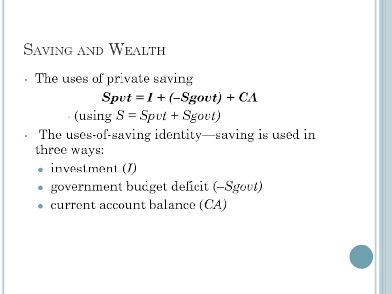
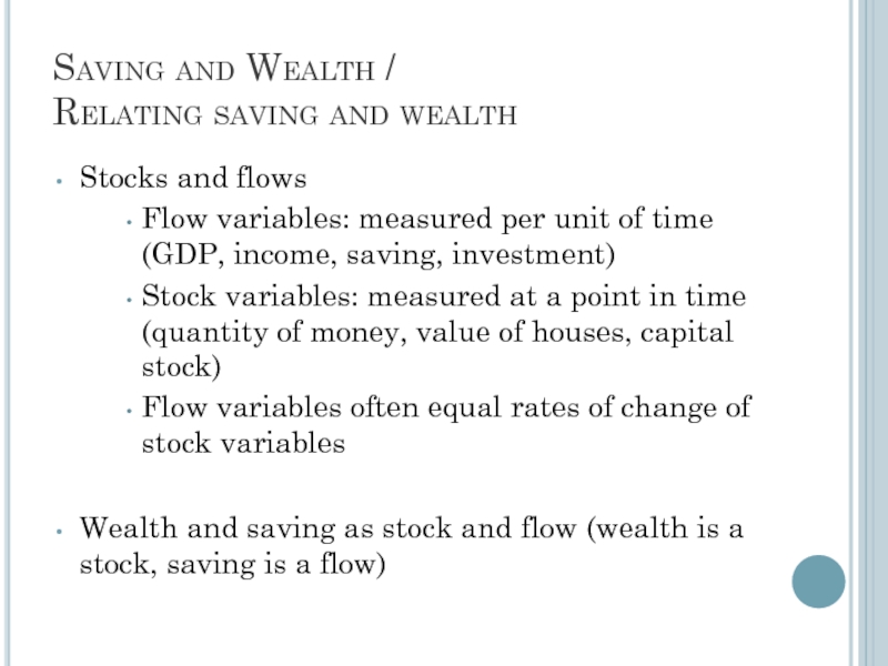
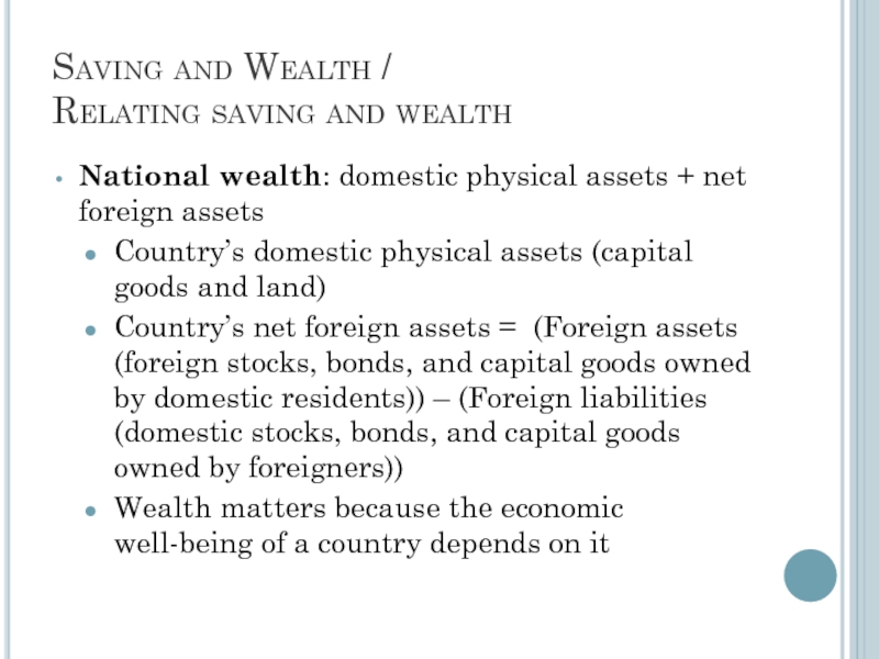
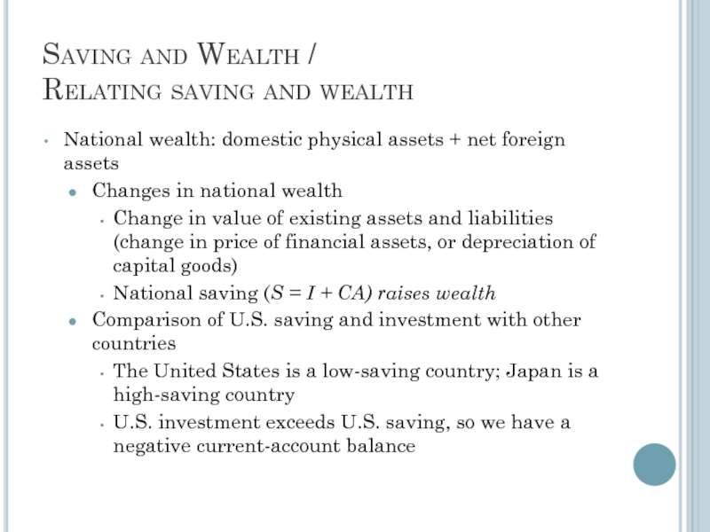
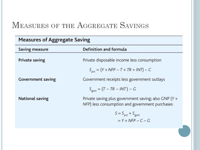
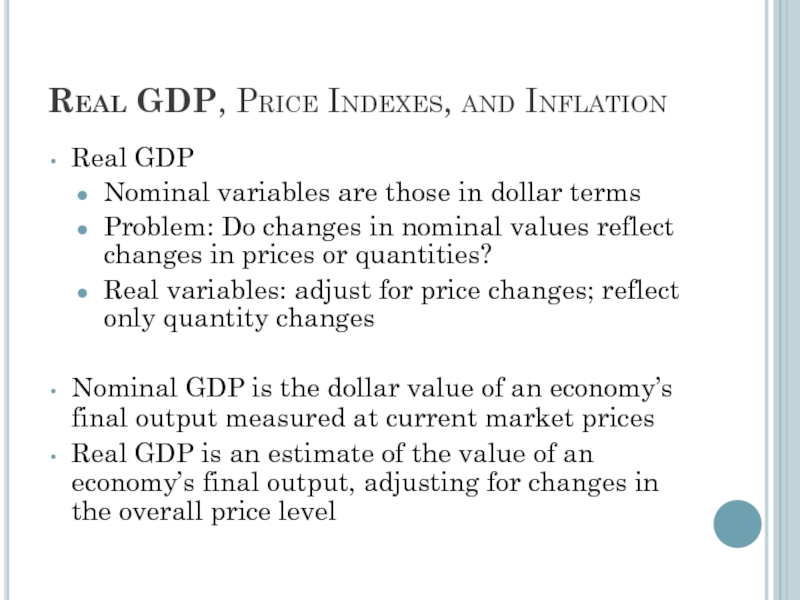

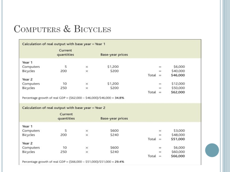
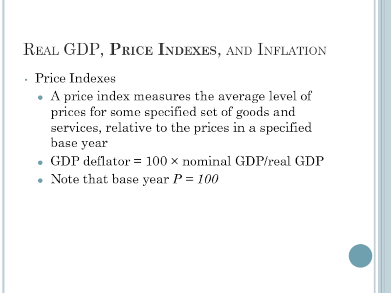
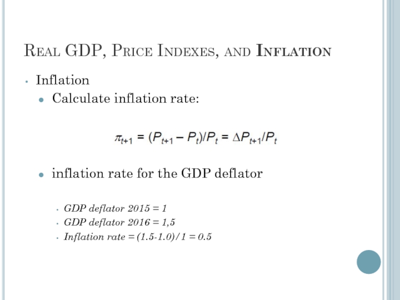

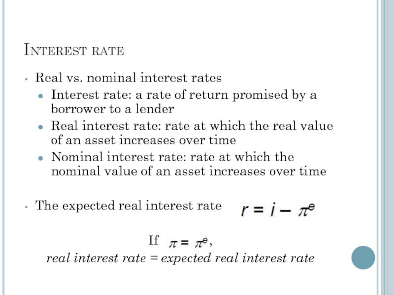





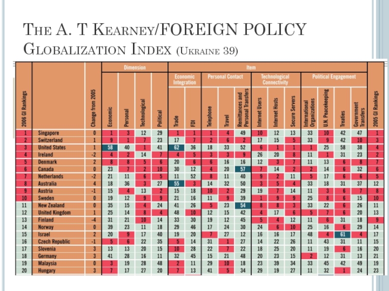
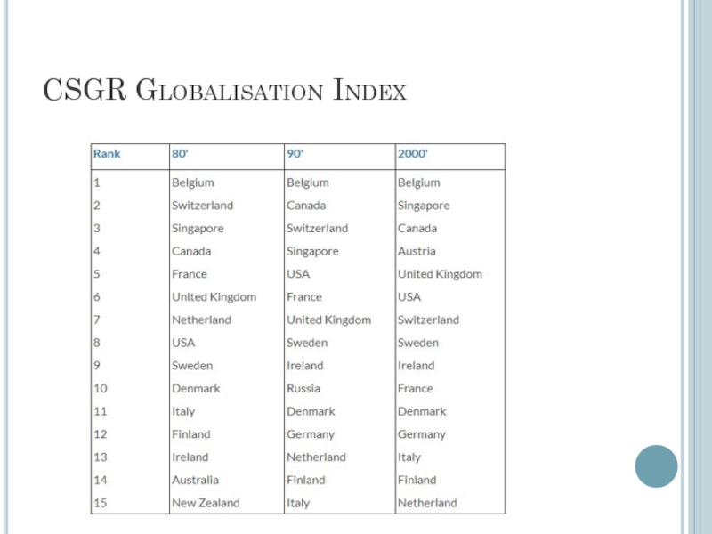
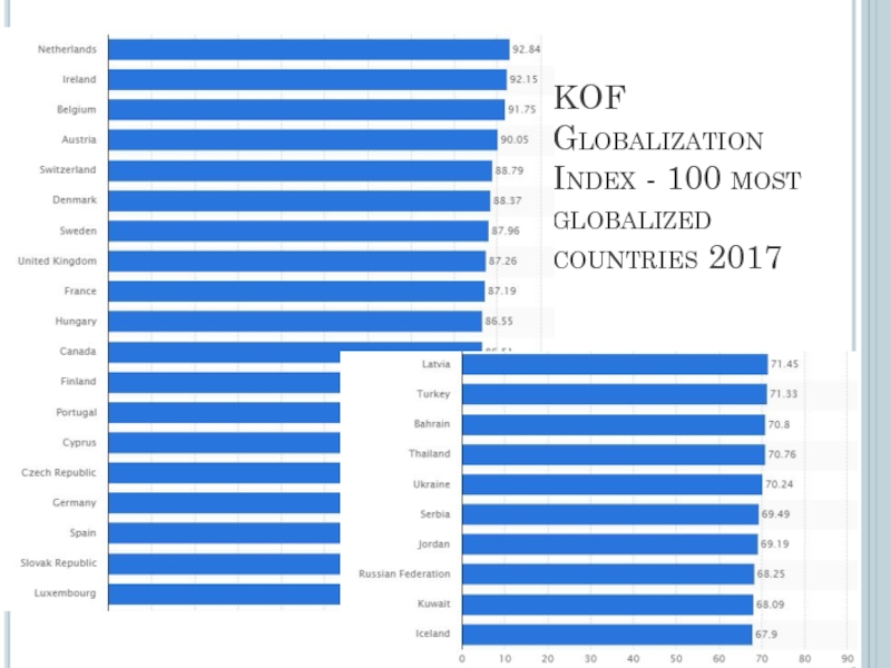
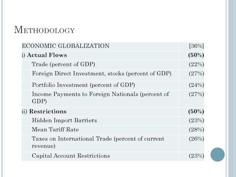
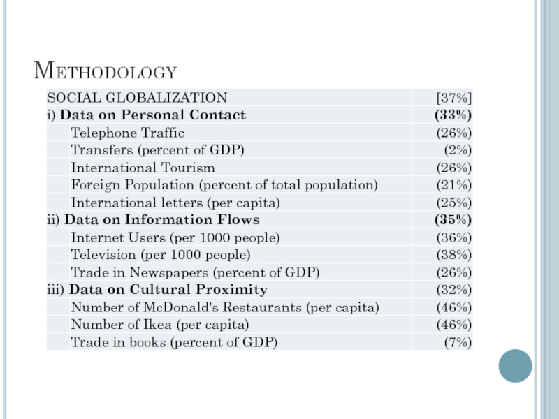
![MethodologyPOLITICAL GLOBALIZATION [27%] Embassies in Country (25%) Membership in International Organizations (27%) Participation in U.N. Security Council Missions (22%) International Treaties (26%)](/img/tmb/4/362034/e7ff30b0c9dc4b20476d6d95bb55f451-800x.jpg)

