- Главная
- Разное
- Дизайн
- Бизнес и предпринимательство
- Аналитика
- Образование
- Развлечения
- Красота и здоровье
- Финансы
- Государство
- Путешествия
- Спорт
- Недвижимость
- Армия
- Графика
- Культурология
- Еда и кулинария
- Лингвистика
- Английский язык
- Астрономия
- Алгебра
- Биология
- География
- Детские презентации
- Информатика
- История
- Литература
- Маркетинг
- Математика
- Медицина
- Менеджмент
- Музыка
- МХК
- Немецкий язык
- ОБЖ
- Обществознание
- Окружающий мир
- Педагогика
- Русский язык
- Технология
- Физика
- Философия
- Химия
- Шаблоны, картинки для презентаций
- Экология
- Экономика
- Юриспруденция
Image Stitching презентация
Содержание
- 1. Image Stitching
- 2. Combine two or more overlapping images to
- 3. How to do it? Basic Procedure Take
- 4. 1. Take a sequence of images from
- 5. 2. Compute transformation between images Extract interest
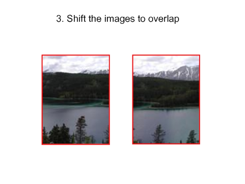
- 6. 3. Shift the images to overlap
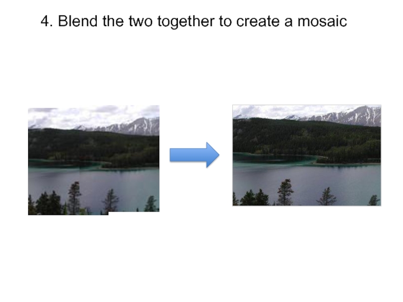
- 7. 4. Blend the two together to create a mosaic
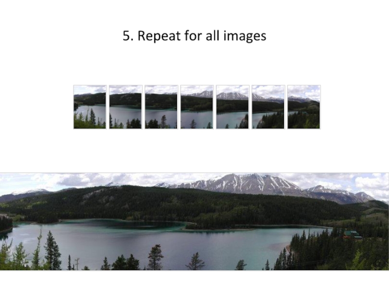
- 8. 5. Repeat for all images
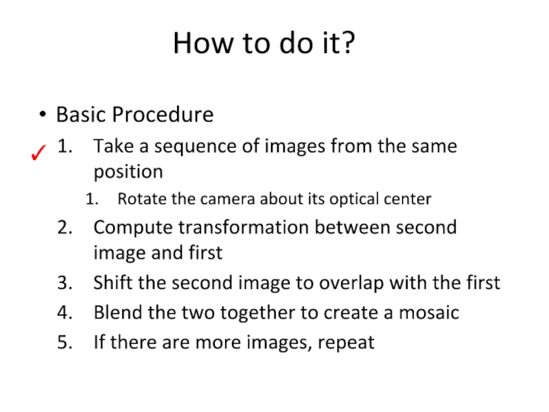
- 9. How to do it? Basic Procedure Take
- 10. Compute Transformations Extract interest points Find good
- 11. Image reprojection The mosaic has a natural
- 12. Example Camera Center
- 13. Image reprojection Observation Rather than thinking of
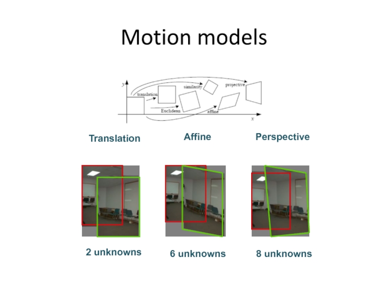
- 14. Motion models What happens when we take
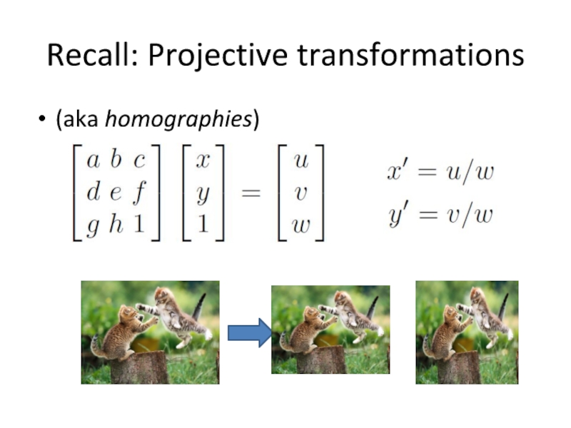
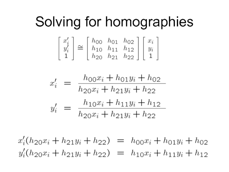
- 15. Recall: Projective transformations (aka homographies)
- 16. Parametric (global) warping Examples of parametric warps: translation rotation aspect affine perspective
- 17. 2D coordinate transformations translation: x’ = x +
- 18. Image Warping Given a coordinate transform x’
- 19. Forward Warping Send each pixel f(x) to
- 20. Forward Warping Send each pixel f(x) to
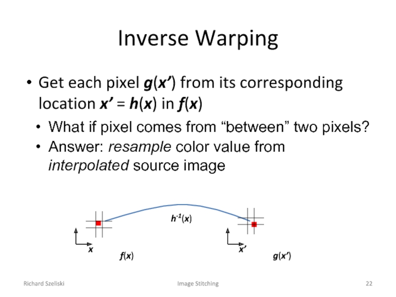
- 21. Richard Szeliski Image Stitching Inverse Warping Get
- 22. Richard Szeliski Image Stitching Inverse Warping Get
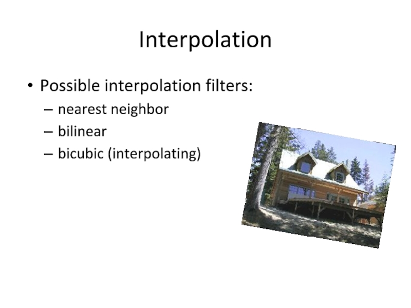
- 23. Interpolation Possible interpolation filters: nearest neighbor bilinear bicubic (interpolating)
- 24. Motion models
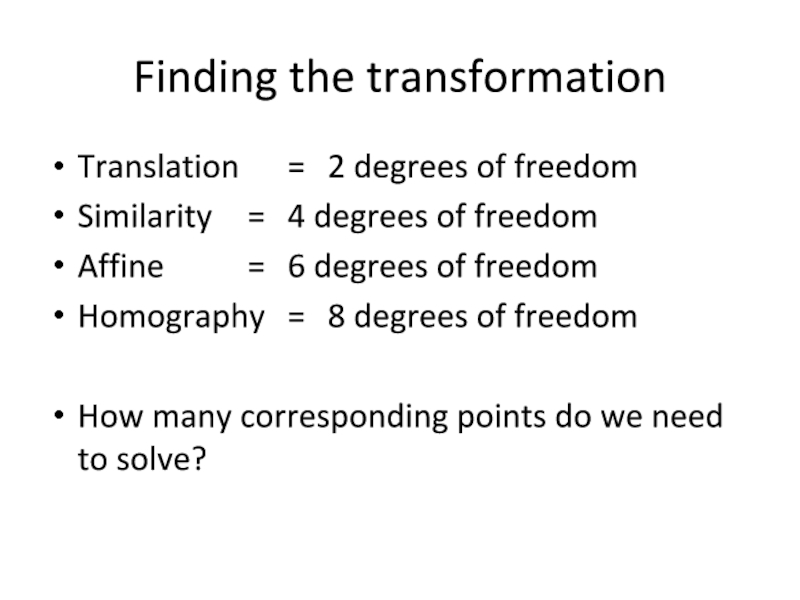
- 25. Finding the transformation Translation = 2 degrees
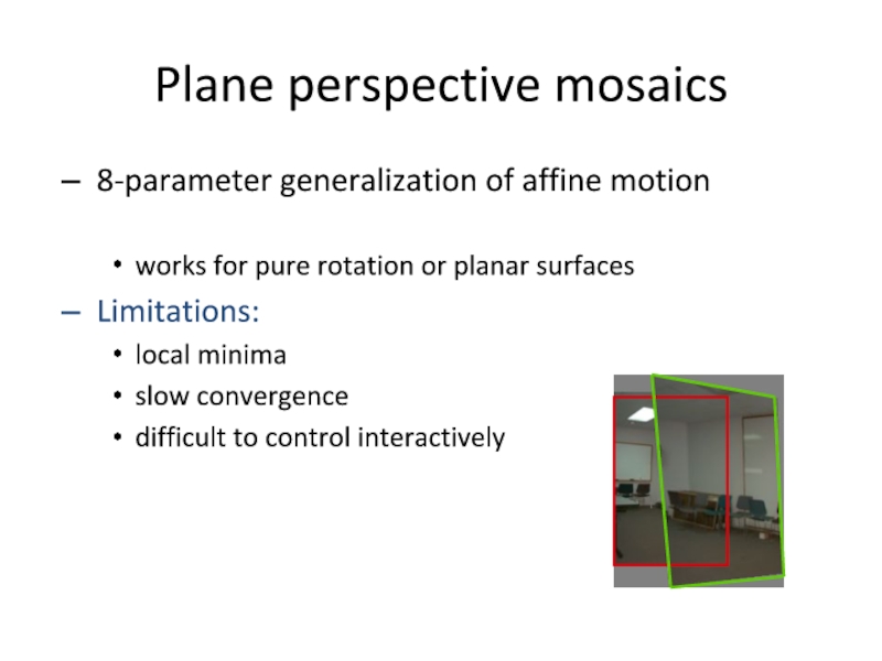
- 26. Plane perspective mosaics 8-parameter generalization of affine
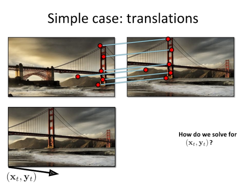
- 27. Simple case: translations
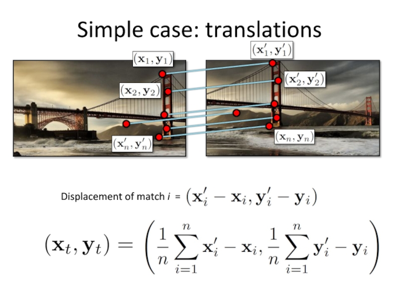
- 28. Simple case: translations
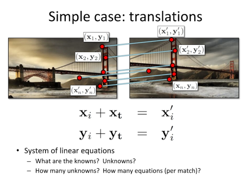
- 29. Simple case: translations System of linear equations
- 30. Simple case: translations Problem: more equations than
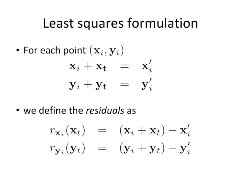
- 31. Least squares formulation For each point we define the residuals as
- 32. Least squares formulation Goal: minimize sum of
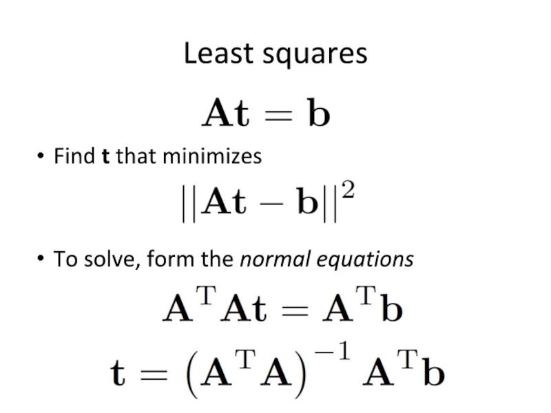
- 33. Least squares Find t that minimizes To solve, form the normal equations
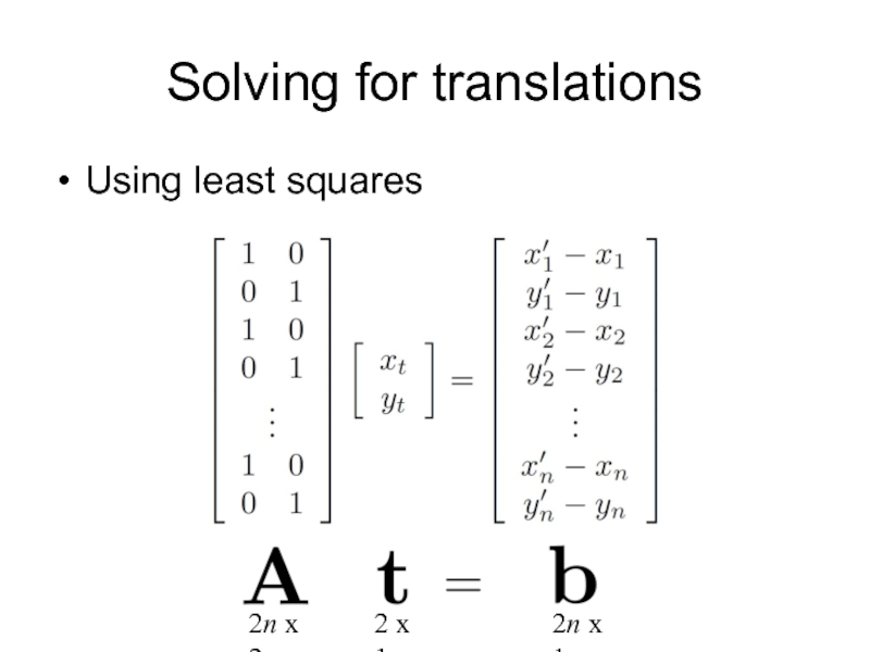
- 34. Solving for translations Using least squares
- 35. Affine transformations How many unknowns? How many
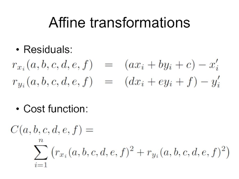
- 36. Affine transformations Residuals: Cost function:
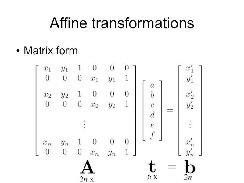
- 37. Affine transformations Matrix form
- 38. Solving for homographies
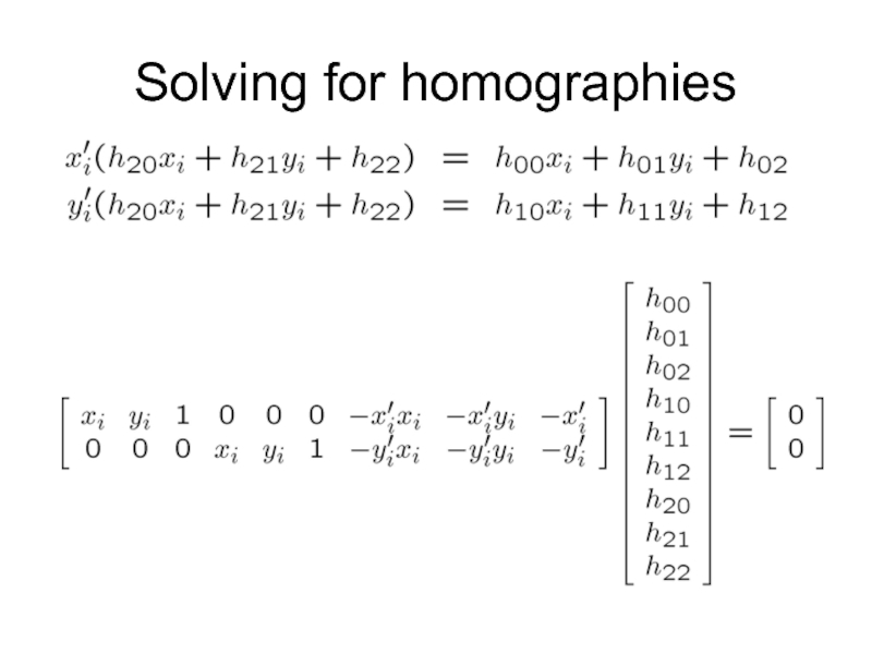
- 39. Solving for homographies
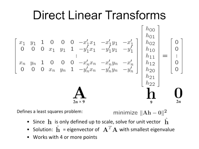
- 40. Direct Linear Transforms Defines a least squares
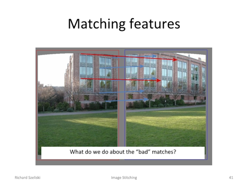
- 41. Richard Szeliski Image Stitching Matching features What do we do about the “bad” matches?
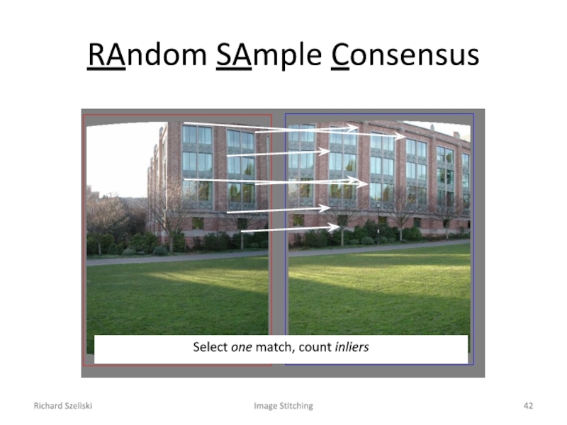
- 42. Richard Szeliski Image Stitching RAndom SAmple Consensus Select one match, count inliers
- 43. Richard Szeliski Image Stitching RAndom SAmple Consensus Select one match, count inliers
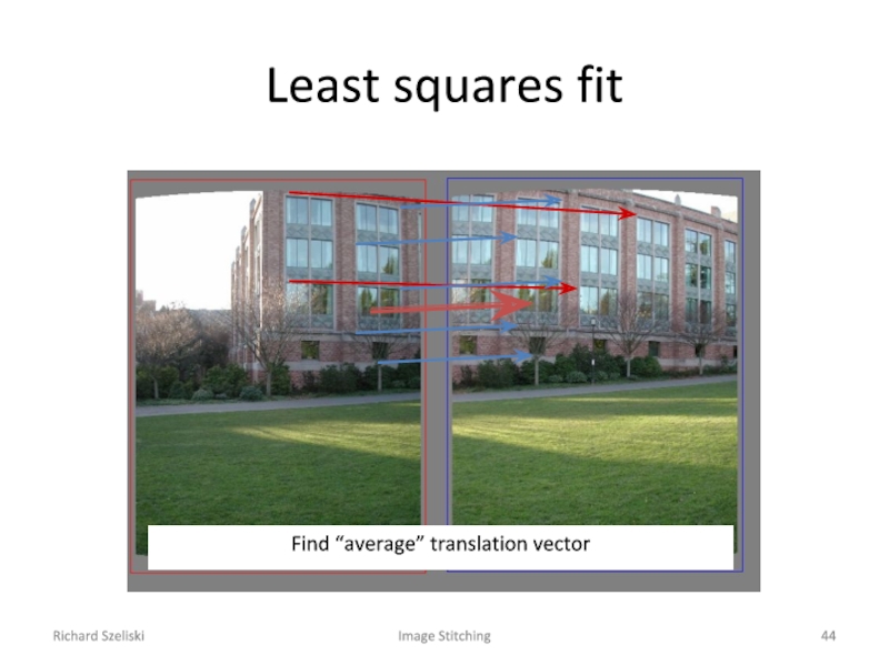
- 44. Richard Szeliski Image Stitching Least squares fit Find “average” translation vector
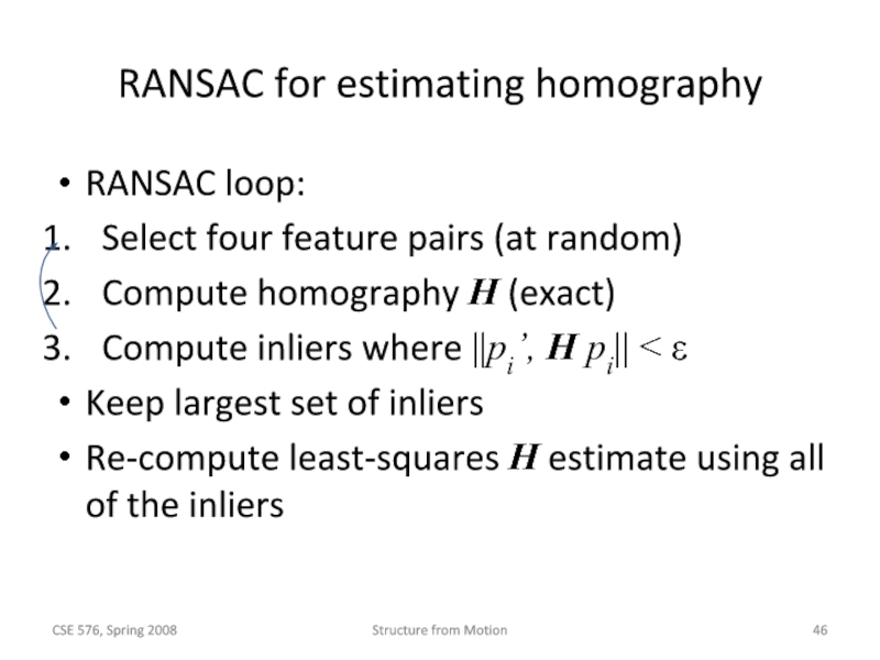
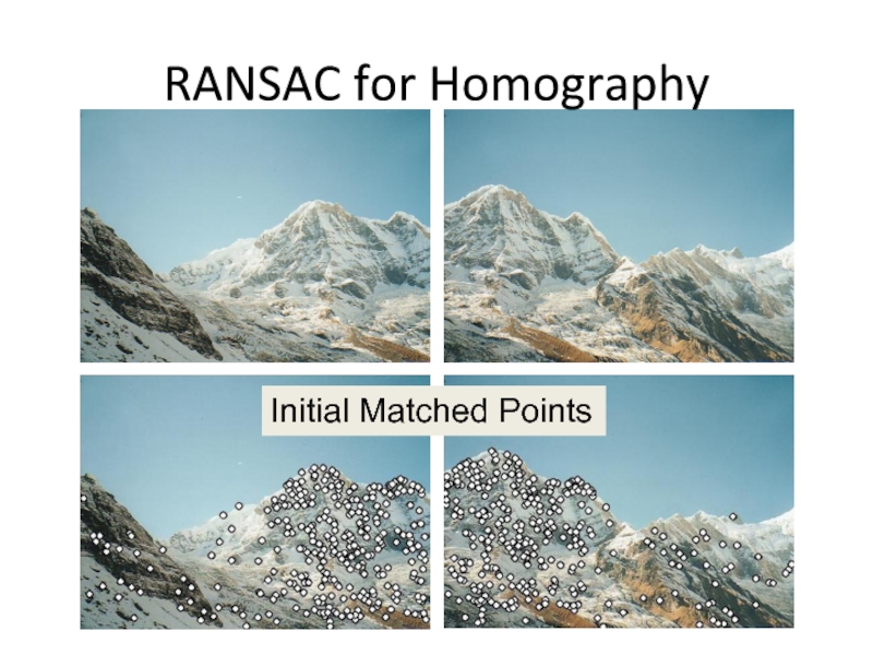
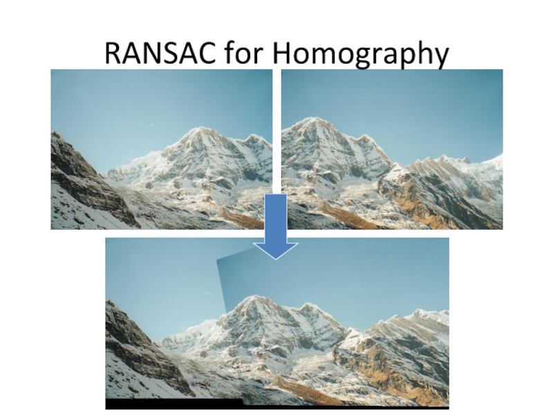
- 46. RANSAC for estimating homography RANSAC loop: Select
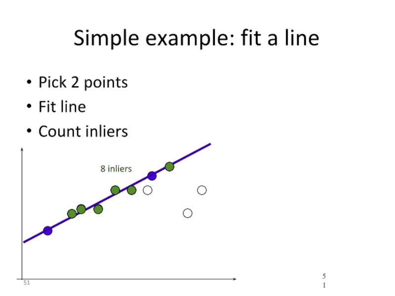
- 47. Simple example: fit a line Rather than
- 48. Simple example: fit a line Pick 2
- 49. Simple example: fit a line Pick 2
- 50. Simple example: fit a line Pick 2
- 51. Simple example: fit a line Pick 2
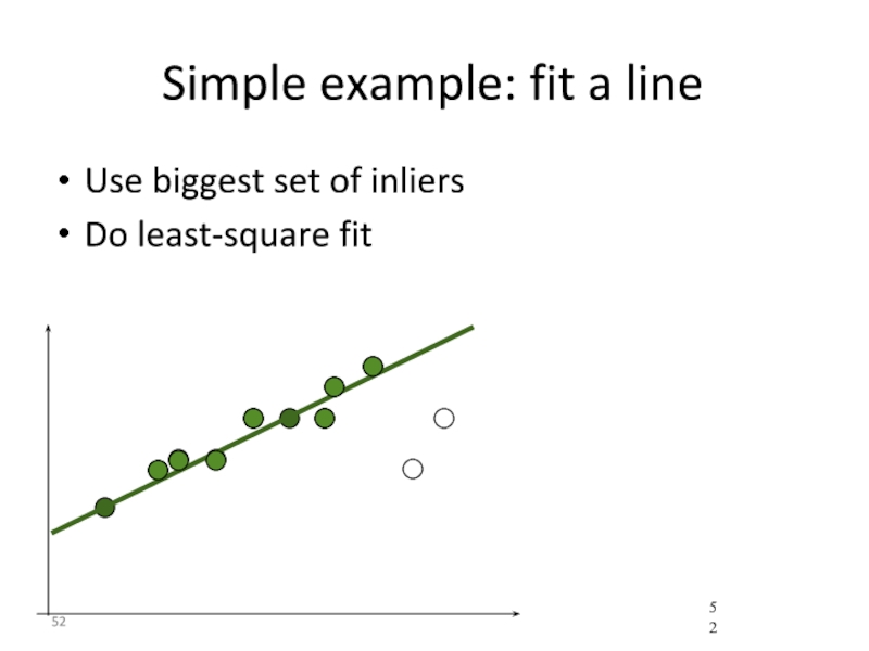
- 52. Simple example: fit a line Use biggest
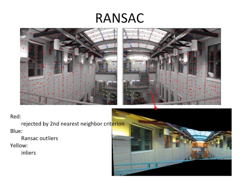
- 53. RANSAC Red: rejected by 2nd nearest neighbor criterion Blue: Ransac outliers Yellow: inliers
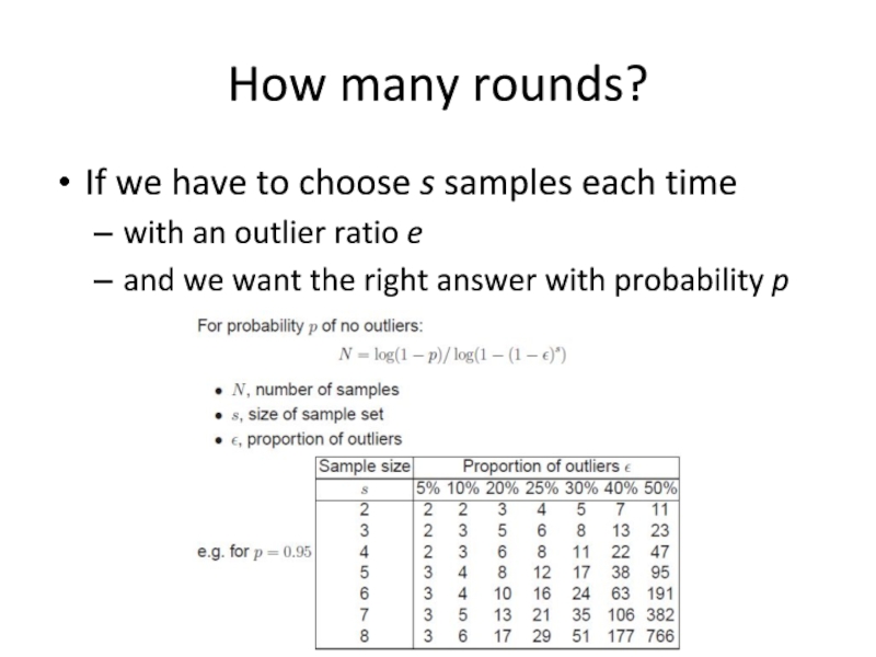
- 54. How many rounds? If we have
- 55. Richard Szeliski Image Stitching Rotational mosaics Directly
- 56. Richard Szeliski Image Stitching Rotational mosaic Projection
- 57. Computing homography Assume we have four matched
- 58. Computing homography Assume we have matched points
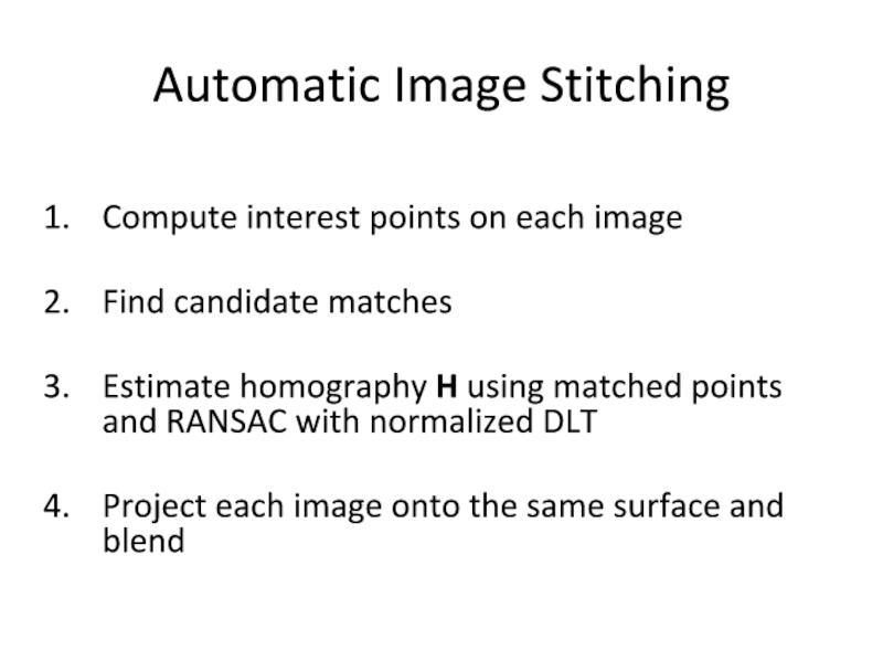
- 59. Automatic Image Stitching Compute interest points
- 60. RANSAC for Homography Initial Matched Points
- 61. RANSAC for Homography Final Matched Points
- 62. RANSAC for Homography
Слайд 1Image Stitching
Ali Farhadi
CSE 455
Several slides from Rick Szeliski, Steve Seitz, Derek
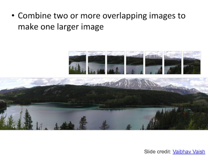
Слайд 2Combine two or more overlapping images to make one larger image
Add
Slide credit: Vaibhav Vaish
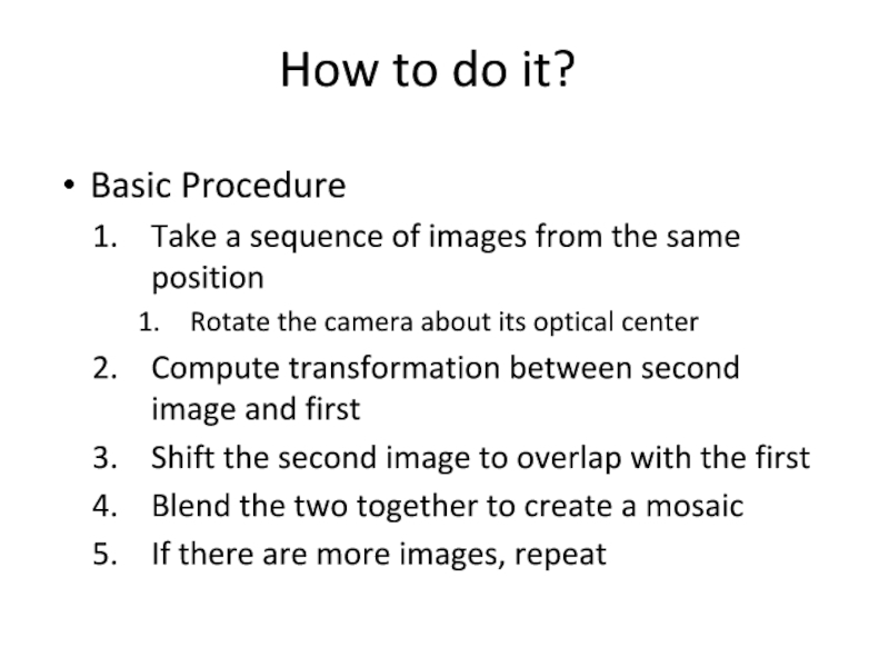
Слайд 3How to do it?
Basic Procedure
Take a sequence of images from the
Rotate the camera about its optical center
Compute transformation between second image and first
Shift the second image to overlap with the first
Blend the two together to create a mosaic
If there are more images, repeat
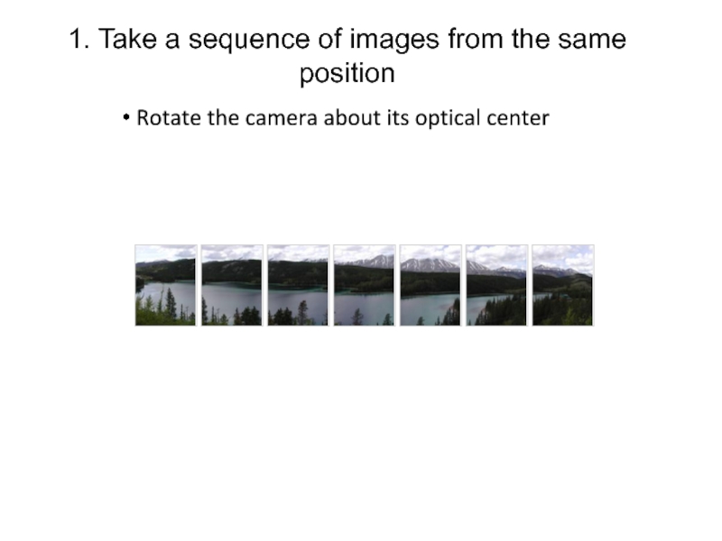
Слайд 41. Take a sequence of images from the same position
Rotate the
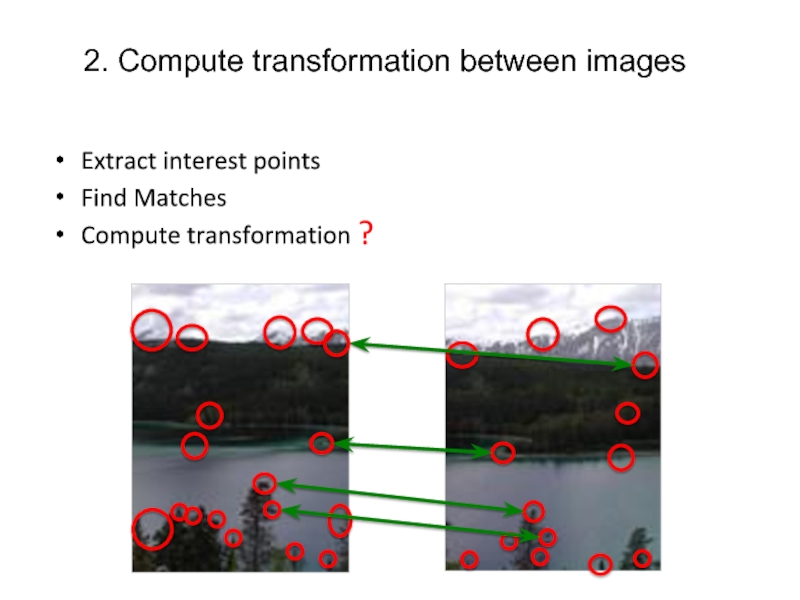
Слайд 52. Compute transformation between images
Extract interest points
Find Matches
Compute transformation
?
Слайд 9How to do it?
Basic Procedure
Take a sequence of images from the
Rotate the camera about its optical center
Compute transformation between second image and first
Shift the second image to overlap with the first
Blend the two together to create a mosaic
If there are more images, repeat
✓
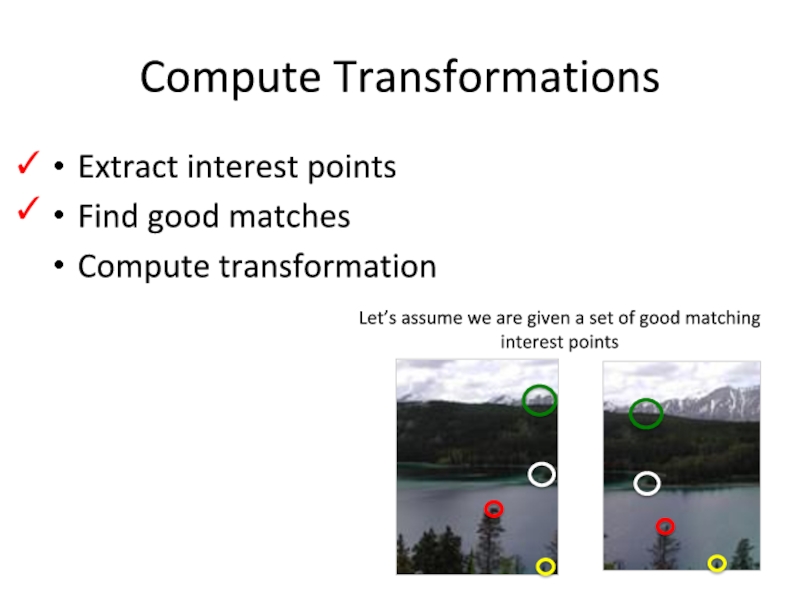
Слайд 10Compute Transformations
Extract interest points
Find good matches
Compute transformation
✓
Let’s assume we are
✓
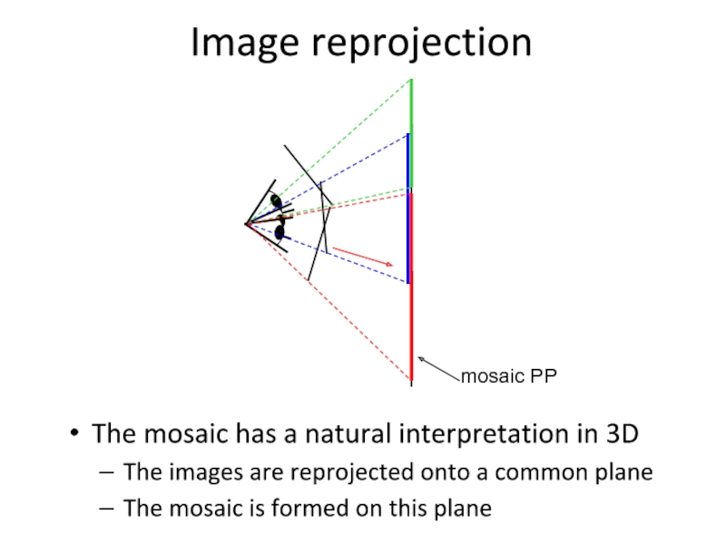
Слайд 11Image reprojection
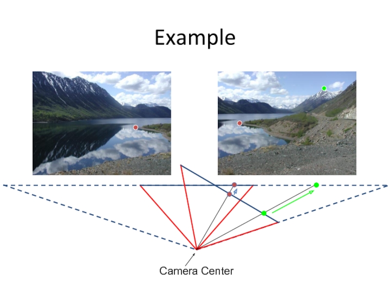
The mosaic has a natural interpretation in 3D
The images are
The mosaic is formed on this plane
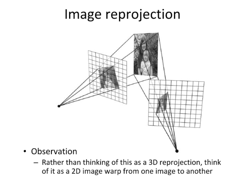
Слайд 13Image reprojection
Observation
Rather than thinking of this as a 3D reprojection, think
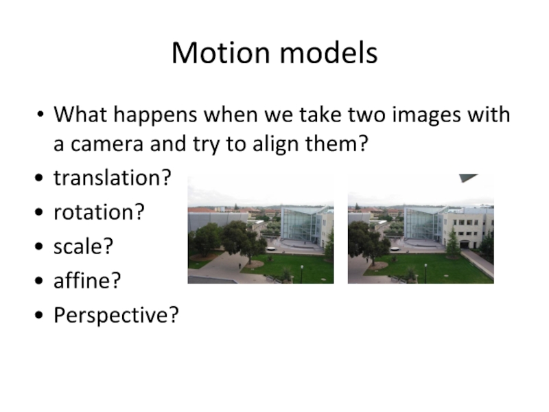
Слайд 14Motion models
What happens when we take two images with a camera
translation?
rotation?
scale?
affine?
Perspective?
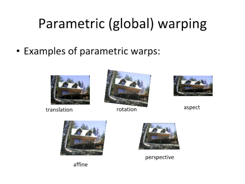
Слайд 16Parametric (global) warping
Examples of parametric warps:
translation
rotation
aspect
affine
perspective
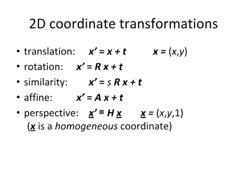
Слайд 172D coordinate transformations
translation: x’ = x + t x = (x,y)
rotation: x’ =
similarity: x’ = s R x + t
affine: x’ = A x + t
perspective: x’ ≅ H x x = (x,y,1) (x is a homogeneous coordinate)
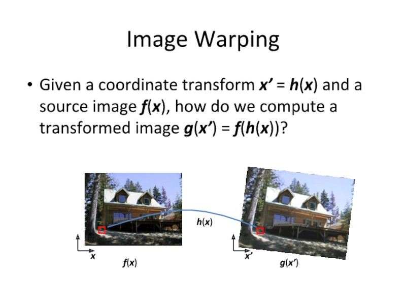
Слайд 18Image Warping
Given a coordinate transform x’ = h(x) and a source
f(x)
g(x’)
x
x’
h(x)
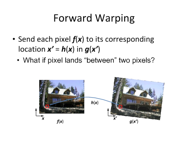
Слайд 19Forward Warping
Send each pixel f(x) to its corresponding location x’ =
f(x)
g(x’)
x
x’
h(x)
What if pixel lands “between” two pixels?
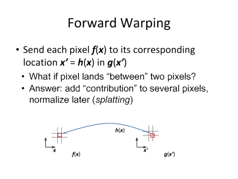
Слайд 20Forward Warping
Send each pixel f(x) to its corresponding location x’ =
f(x)
g(x’)
x
x’
h(x)
What if pixel lands “between” two pixels?
Answer: add “contribution” to several pixels, normalize later (splatting)
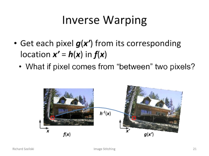
Слайд 21Richard Szeliski
Image Stitching
Inverse Warping
Get each pixel g(x’) from its corresponding location
f(x)
g(x’)
x
x’
h-1(x)
What if pixel comes from “between” two pixels?
Слайд 22Richard Szeliski
Image Stitching
Inverse Warping
Get each pixel g(x’) from its corresponding location
What if pixel comes from “between” two pixels?
Answer: resample color value from interpolated source image
f(x)
g(x’)
x
x’
h-1(x)
Слайд 25Finding the transformation
Translation = 2 degrees of freedom
Similarity = 4 degrees
Affine = 6 degrees of freedom
Homography = 8 degrees of freedom
How many corresponding points do we need to solve?
Слайд 26Plane perspective mosaics
8-parameter generalization of affine motion
works for pure rotation or
Limitations:
local minima
slow convergence
difficult to control interactively
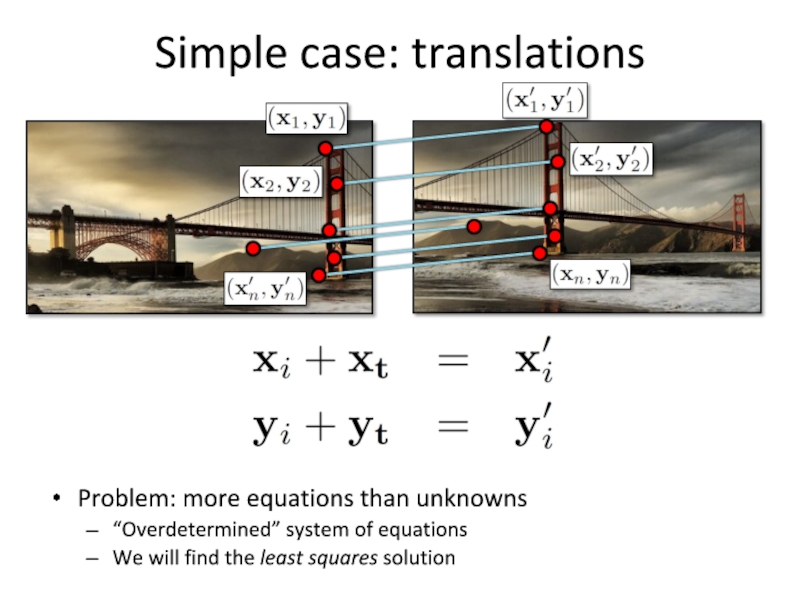
Слайд 29Simple case: translations
System of linear equations
What are the knowns? Unknowns?
How many
Слайд 30Simple case: translations
Problem: more equations than unknowns
“Overdetermined” system of equations
We will
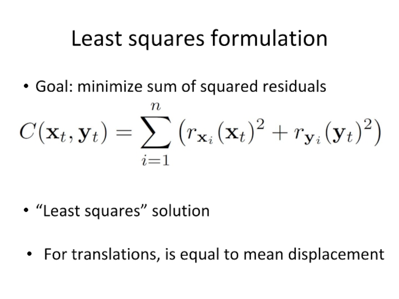
Слайд 32Least squares formulation
Goal: minimize sum of squared residuals
“Least squares” solution
For translations,
Слайд 35Affine transformations
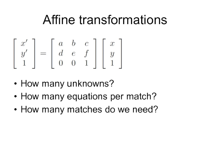
How many unknowns?
How many equations per match?
How many matches do
Слайд 40Direct Linear Transforms
Defines a least squares problem:
Since is
Solution: = eigenvector of with smallest eigenvalue
Works with 4 or more points
Слайд 46RANSAC for estimating homography
RANSAC loop:
Select four feature pairs (at random)
Compute homography
Compute inliers where ||pi’, H pi|| < ε
Keep largest set of inliers
Re-compute least-squares H estimate using all of the inliers
CSE 576, Spring 2008
Structure from Motion
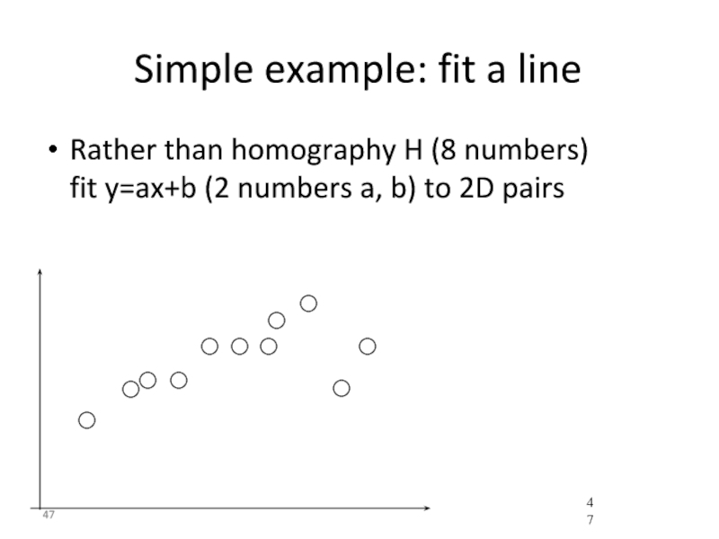
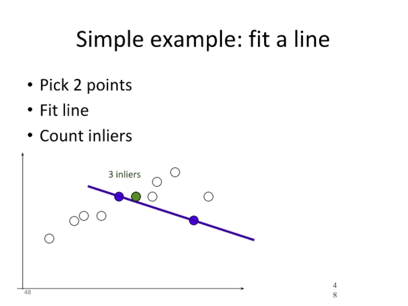
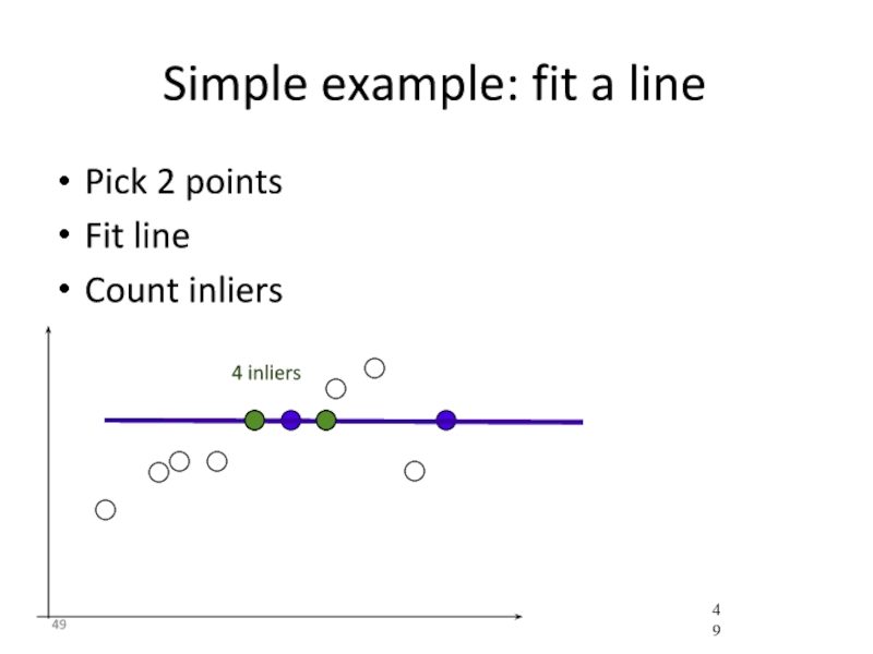
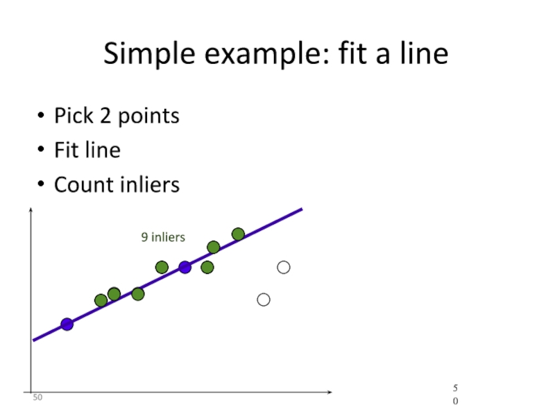
Слайд 47Simple example: fit a line
Rather than homography H (8 numbers)
fit
Слайд 54How many rounds?
If we have to choose s samples each
with an outlier ratio e
and we want the right answer with probability p
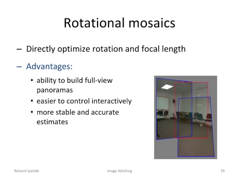
Слайд 55Richard Szeliski
Image Stitching
Rotational mosaics
Directly optimize rotation and focal length
Advantages:
ability to build
easier to control interactively
more stable and accurate estimates
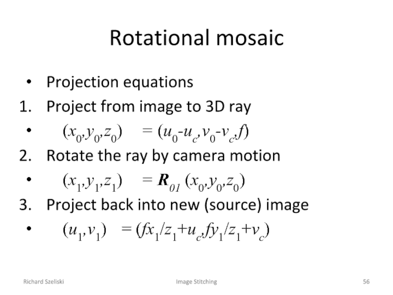
Слайд 56Richard Szeliski
Image Stitching
Rotational mosaic
Projection equations
Project from image to 3D ray
(x0,y0,z0) =
Rotate the ray by camera motion
(x1,y1,z1) = R01 (x0,y0,z0)
Project back into new (source) image
(u1,v1) = (fx1/z1+uc,fy1/z1+vc)
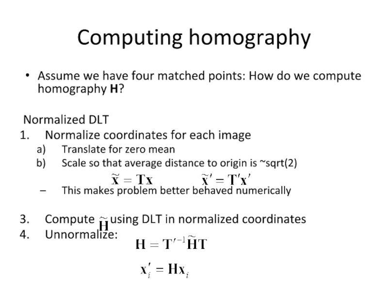
Слайд 57Computing homography
Assume we have four matched points: How do we compute
Normalized DLT
Normalize coordinates for each image
Translate for zero mean
Scale so that average distance to origin is ~sqrt(2)
This makes problem better behaved numerically
Compute using DLT in normalized coordinates
Unnormalize:
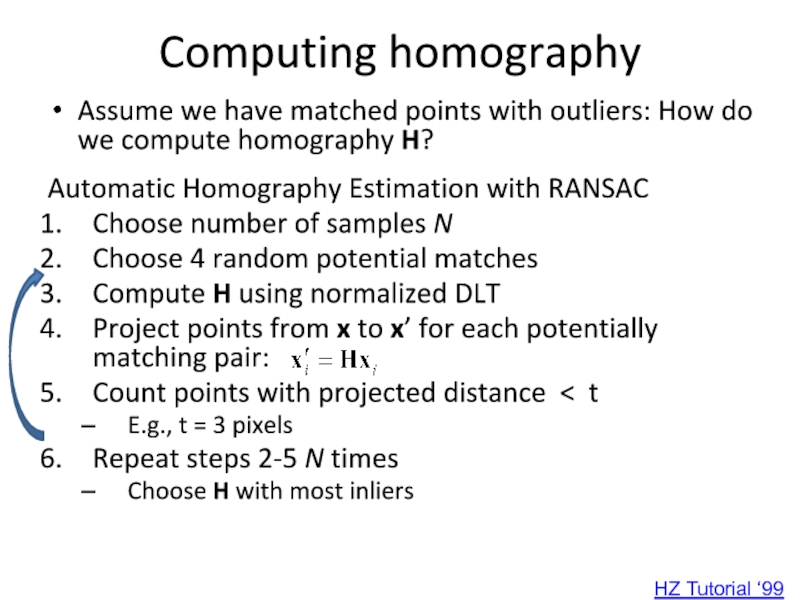
Слайд 58Computing homography
Assume we have matched points with outliers: How do we
Automatic Homography Estimation with RANSAC
Choose number of samples N
Choose 4 random potential matches
Compute H using normalized DLT
Project points from x to x’ for each potentially matching pair:
Count points with projected distance < t
E.g., t = 3 pixels
Repeat steps 2-5 N times
Choose H with most inliers
HZ Tutorial ‘99
Слайд 59Automatic Image Stitching
Compute interest points on each image
Find candidate matches
Estimate homography
Project each image onto the same surface and blend
