- Главная
- Разное
- Дизайн
- Бизнес и предпринимательство
- Аналитика
- Образование
- Развлечения
- Красота и здоровье
- Финансы
- Государство
- Путешествия
- Спорт
- Недвижимость
- Армия
- Графика
- Культурология
- Еда и кулинария
- Лингвистика
- Английский язык
- Астрономия
- Алгебра
- Биология
- География
- Детские презентации
- Информатика
- История
- Литература
- Маркетинг
- Математика
- Медицина
- Менеджмент
- Музыка
- МХК
- Немецкий язык
- ОБЖ
- Обществознание
- Окружающий мир
- Педагогика
- Русский язык
- Технология
- Физика
- Философия
- Химия
- Шаблоны, картинки для презентаций
- Экология
- Экономика
- Юриспруденция
Financial Econometrics II презентация
Содержание
- 1. Financial Econometrics II
- 2. Up to now: Event study analysis:
- 3. Plan for today: Advanced topic: event
- 4. How to measure average reaction to the
- 5. What if the event date is uncertain?
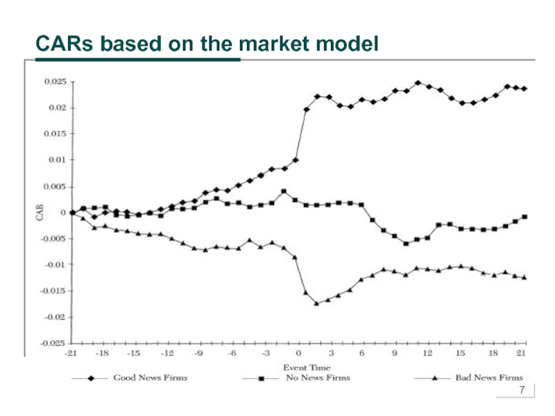
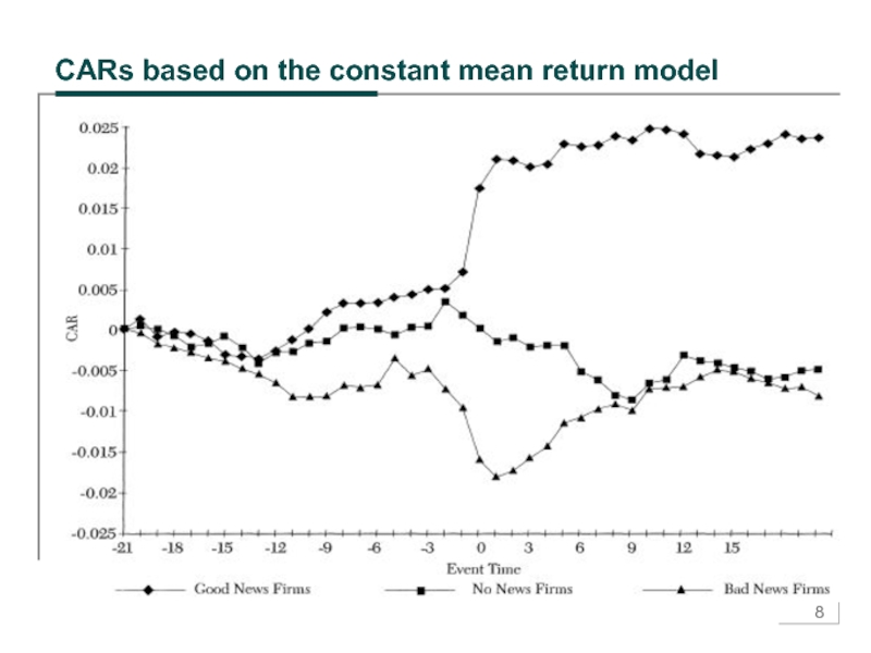
- 6. Example: reaction to earnings announcements CLM, Table
- 7. CARs based on the market model
- 8. CARs based on the constant mean return model
- 9. Methodology: explaining abnormal returns Relation between
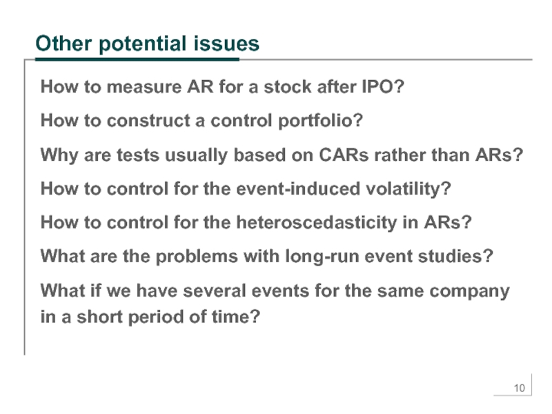
- 10. Other potential issues How to measure
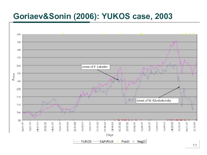
- 11. Goriaev&Sonin (2006): YUKOS case, 2003
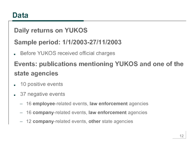
- 12. Data Daily returns on YUKOS Sample period:
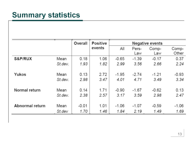
- 13. Summary statistics
- 14. How did YUKOS stock react to events?
- 15. How did YUKOS stock react to events?
- 16. How did other companies react to YUKOS
- 17. How did other companies react to YUKOS events?
- 18. Conclusions Russian firms were very sensitive to
- 19. Other examples of event studies Security offerings
- 20. Strengths of the event study analysis Direct
- 21. Why beta? Main conclusion from tests of
- 22. CAPM vs. the market model Time series
- 23. Use of the market model Ri,t =
- 24. Estimating beta β=cov(Ri, RM)/var(RM) In Excel (see
- 25. Is historical beta a good predictor of
- 26. How are betas correlated over time?
- 27. Mean reversion in betas
- 28. Autoregression of betas
- 29. Vasicek’s adjustment Bayesian adjustment, Vasicek (1973): The
- 30. Estimating beta for illiquid stocks Assume that
- 31. Estimating beta for illiquid stocks The “trade-to-trade”
- 32. What if the stock has a large
- 33. Fundamental beta Can we explain betas by
- 34. Next class Advanced topic: testing CAPM Is
Слайд 2Up to now:
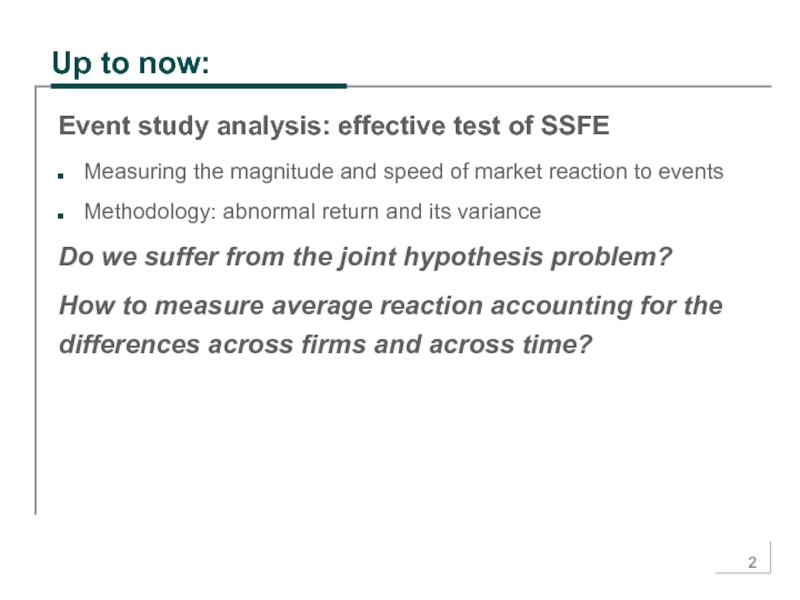
Event study analysis: effective test of SSFE
Measuring the
magnitude and speed of market reaction to events
Methodology: abnormal return and its variance
Do we suffer from the joint hypothesis problem?
How to measure average reaction accounting for the differences across firms and across time?
Methodology: abnormal return and its variance
Do we suffer from the joint hypothesis problem?
How to measure average reaction accounting for the differences across firms and across time?
Слайд 3Plan for today:
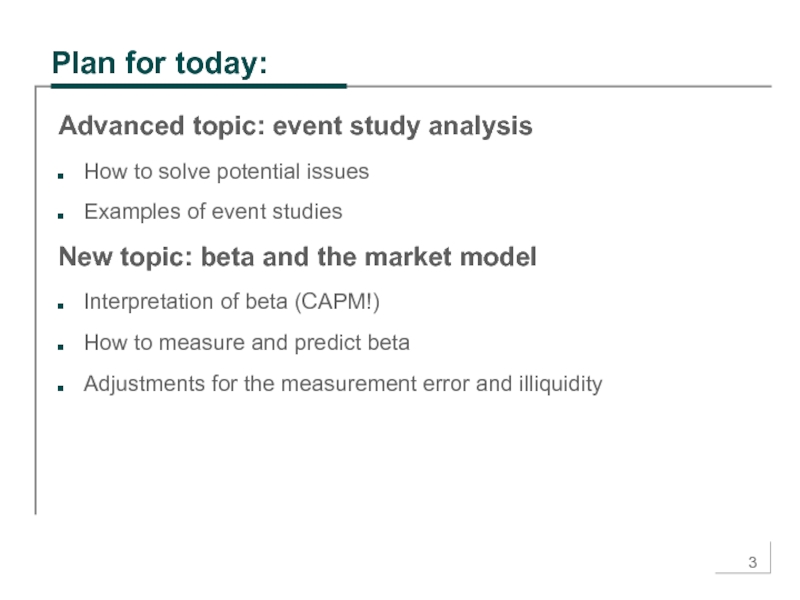
Advanced topic: event study analysis
How to solve potential
issues
Examples of event studies
New topic: beta and the market model
Interpretation of beta (CAPM!)
How to measure and predict beta
Adjustments for the measurement error and illiquidity
Examples of event studies
New topic: beta and the market model
Interpretation of beta (CAPM!)
How to measure and predict beta
Adjustments for the measurement error and illiquidity
Слайд 4How to measure average reaction to the event?
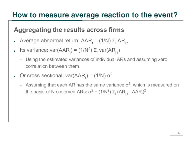
Aggregating the results across
firms
Average abnormal return: AARt = (1/N) Σi ARi,t
Its variance: var(AARt) = (1/N2) Σi var(ARi,t)
Using the estimated variances of individual ARs and assuming zero correlation between them
Or cross-sectional: var(AARt) = (1/N) σ2
Assuming that each AR has the same variance σ2, which is measured on the basis of N observed ARs: σ2 = (1/N2) Σi (ARi,t - AARt)2
Слайд 5What if the event date is uncertain?
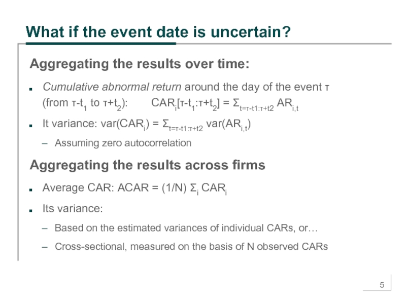
Aggregating the results over time:
Cumulative abnormal return around the day of the event τ (from τ-t1 to τ+t2): CARi[τ-t1:τ+t2] = Σt=τ-t1:τ+t2 ARi,t
It variance: var(CARi) = Σt=τ-t1:τ+t2 var(ARi,t)
Assuming zero autocorrelation
Aggregating the results across firms
Average CAR: ACAR = (1/N) Σi CARi
Its variance:
Based on the estimated variances of individual CARs, or…
Cross-sectional, measured on the basis of N observed CARs
Слайд 6Example: reaction to earnings announcements
CLM, Table 4.1, Fig 4.2: 30 US
companies, 1989-93
Positive (negative) reaction to good (bad) news at day 0
No significant reaction for no-news
The constant mean return model produces noisier estimates than the market model
Positive (negative) reaction to good (bad) news at day 0
No significant reaction for no-news
The constant mean return model produces noisier estimates than the market model
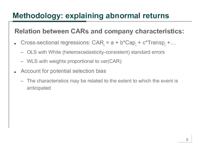
Слайд 9Methodology: explaining abnormal returns
Relation between CARs and company characteristics:
Cross-sectional regressions:
CARi = a + b*Capi + c*Transpi +…
OLS with White (heteroscedasticity-consistent) standard errors
WLS with weights proportional to var(CAR)
Account for potential selection bias
The characteristics may be related to the extent to which the event is anticipated
OLS with White (heteroscedasticity-consistent) standard errors
WLS with weights proportional to var(CAR)
Account for potential selection bias
The characteristics may be related to the extent to which the event is anticipated
Слайд 10Other potential issues
How to measure AR for a stock after
IPO?
How to construct a control portfolio?
Why are tests usually based on CARs rather than ARs?
How to control for the event-induced volatility?
How to control for the heteroscedasticity in ARs?
What are the problems with long-run event studies?
What if we have several events for the same company in a short period of time?
Слайд 12Data
Daily returns on YUKOS
Sample period: 1/1/2003-27/11/2003
Before YUKOS received official charges
Events: publications
mentioning YUKOS and one of the state agencies
10 positive events
37 negative events
16 employee-related events, law enforcement agencies
16 company-related events, law enforcement agencies
12 company-related events, other state agencies
10 positive events
37 negative events
16 employee-related events, law enforcement agencies
16 company-related events, law enforcement agencies
12 company-related events, other state agencies
Слайд 14How did YUKOS stock react to events?
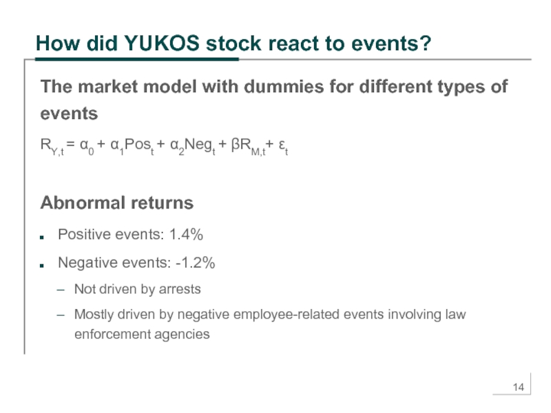
The market model with dummies
for different types of events
RY,t = α0 + α1Post + α2Negt + βRM,t+ εt
Abnormal returns
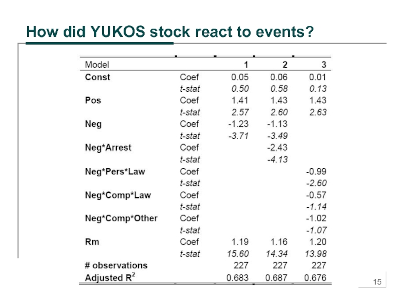
Positive events: 1.4%
Negative events: -1.2%
Not driven by arrests
Mostly driven by negative employee-related events involving law enforcement agencies
RY,t = α0 + α1Post + α2Negt + βRM,t+ εt
Abnormal returns
Positive events: 1.4%
Negative events: -1.2%
Not driven by arrests
Mostly driven by negative employee-related events involving law enforcement agencies
Слайд 16How did other companies react to YUKOS events?
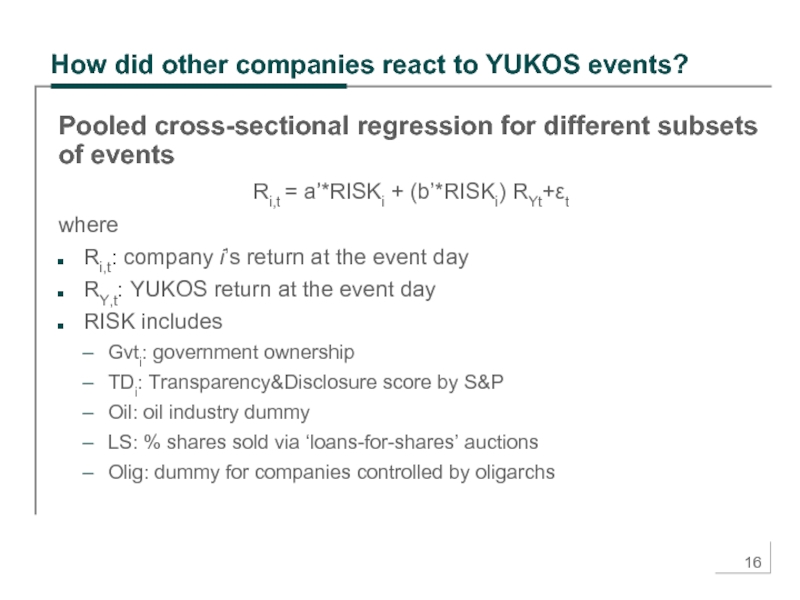
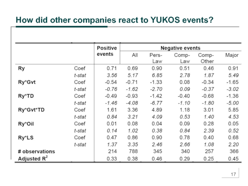
Pooled cross-sectional regression
for different subsets of events
Ri,t = a’*RISKi + (b’*RISKi) RYt+εt
where
Ri,t: company i’s return at the event day
RY,t: YUKOS return at the event day
RISK includes
Gvti: government ownership
TDi: Transparency&Disclosure score by S&P
Oil: oil industry dummy
LS: % shares sold via ‘loans-for-shares’ auctions
Olig: dummy for companies controlled by oligarchs
Слайд 18Conclusions
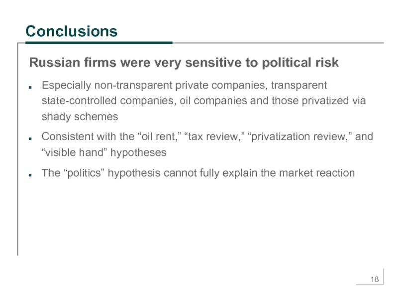
Russian firms were very sensitive to political risk
Especially non-transparent private companies,
transparent state-controlled companies, oil companies and those privatized via shady schemes
Consistent with the “oil rent,” “tax review,” “privatization review,” and “visible hand” hypotheses
The “politics” hypothesis cannot fully explain the market reaction
Consistent with the “oil rent,” “tax review,” “privatization review,” and “visible hand” hypotheses
The “politics” hypothesis cannot fully explain the market reaction
Слайд 19Other examples of event studies
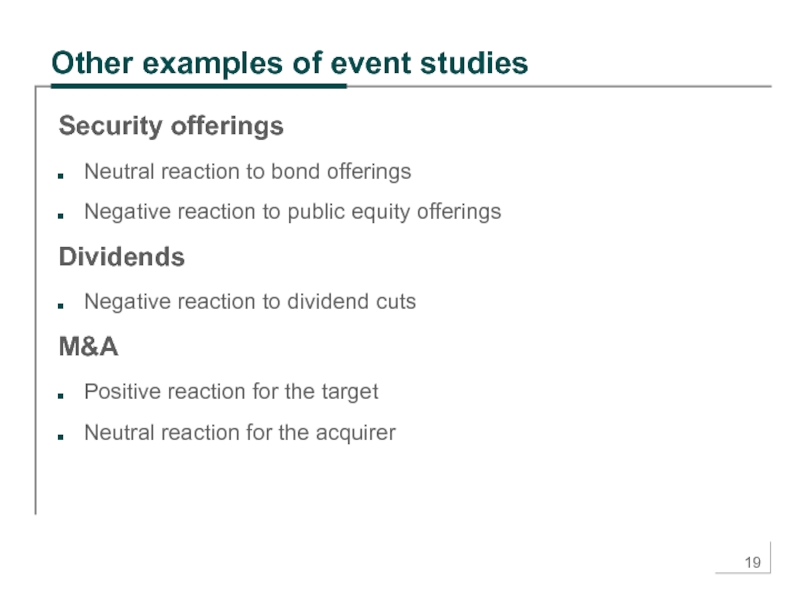
Security offerings
Neutral reaction to bond offerings
Negative reaction
to public equity offerings
Dividends
Negative reaction to dividend cuts
M&A
Positive reaction for the target
Neutral reaction for the acquirer
Dividends
Negative reaction to dividend cuts
M&A
Positive reaction for the target
Neutral reaction for the acquirer
Слайд 20Strengths of the event study analysis
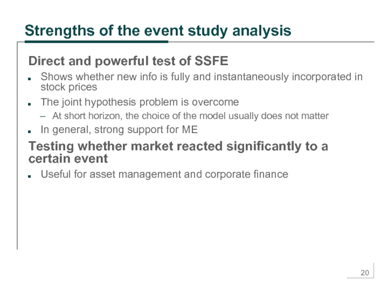
Direct and powerful test of SSFE
Shows
whether new info is fully and instantaneously incorporated in stock prices
The joint hypothesis problem is overcome
At short horizon, the choice of the model usually does not matter
In general, strong support for ME
Testing whether market reacted significantly to a certain event
Useful for asset management and corporate finance
The joint hypothesis problem is overcome
At short horizon, the choice of the model usually does not matter
In general, strong support for ME
Testing whether market reacted significantly to a certain event
Useful for asset management and corporate finance
Слайд 21Why beta?
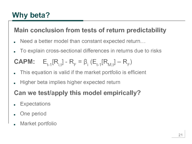
Main conclusion from tests of return predictability
Need a better model
than constant expected return…
To explain cross-sectional differences in returns due to risks
CAPM: Et-1[Ri,t] - RF = βi (Et-1[RM,t] – RF)
This equation is valid if the market portfolio is efficient
Higher beta implies higher expected return
Can we test/apply this model empirically?
Expectations
One period
Market portfolio
To explain cross-sectional differences in returns due to risks
CAPM: Et-1[Ri,t] - RF = βi (Et-1[RM,t] – RF)
This equation is valid if the market portfolio is efficient
Higher beta implies higher expected return
Can we test/apply this model empirically?
Expectations
One period
Market portfolio
Слайд 22CAPM vs. the market model
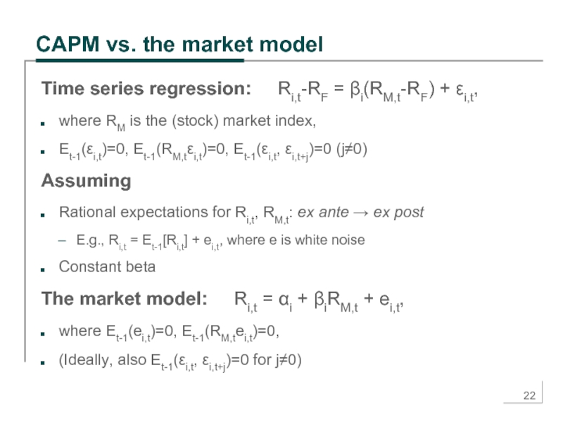
Time series regression: Ri,t-RF =
βi(RM,t-RF) + εi,t,
where RM is the (stock) market index,
Et-1(εi,t)=0, Et-1(RM,tεi,t)=0, Et-1(εi,t, εi,t+j)=0 (j≠0)
Assuming
Rational expectations for Ri,t, RM,t: ex ante → ex post
E.g., Ri,t = Et-1[Ri,t] + ei,t, where e is white noise
Constant beta
The market model: Ri,t = αi + βiRM,t + ei,t,
where Et-1(ei,t)=0, Et-1(RM,tei,t)=0,
(Ideally, also Et-1(εi,t, εi,t+j)=0 for j≠0)
Слайд 23Use of the market model
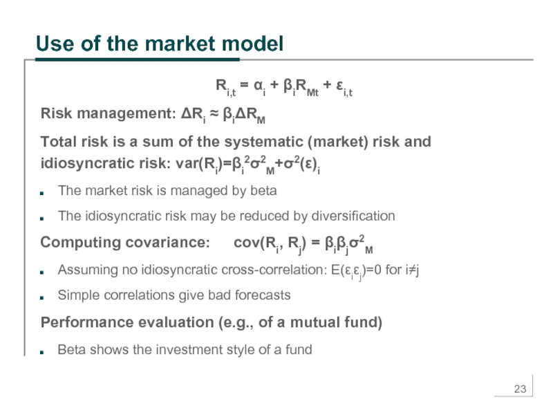
Ri,t = αi + βiRMt + εi,t
Risk
management: ΔRi ≈ βiΔRM
Total risk is a sum of the systematic (market) risk and idiosyncratic risk: var(Ri)=βi2σ2M+σ2(ε)i
The market risk is managed by beta
The idiosyncratic risk may be reduced by diversification
Computing covariance: cov(Ri, Rj) = βiβjσ2M
Assuming no idiosyncratic cross-correlation: E(εiεj)=0 for i≠j
Simple correlations give bad forecasts
Performance evaluation (e.g., of a mutual fund)
Beta shows the investment style of a fund
Слайд 24Estimating beta
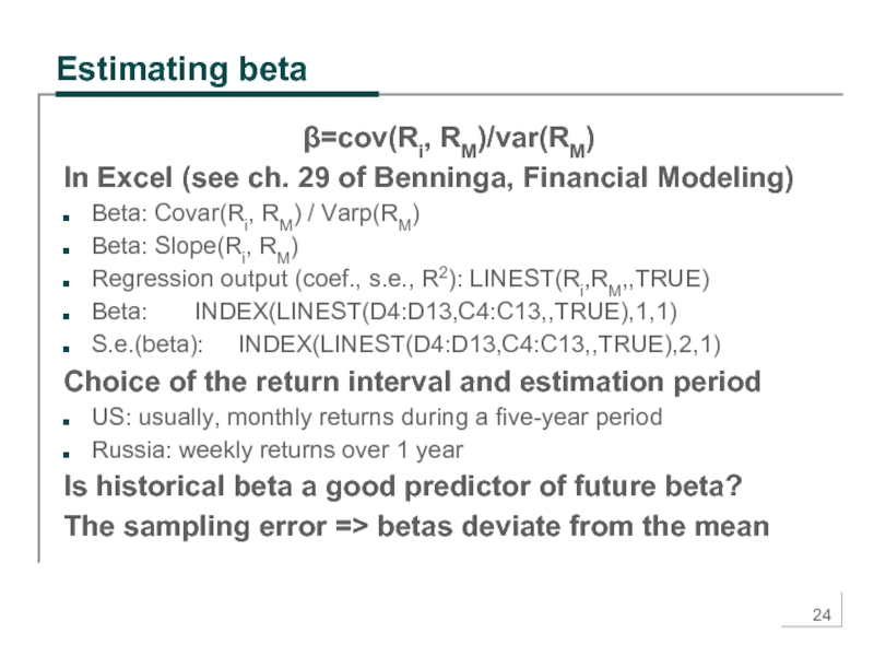
β=cov(Ri, RM)/var(RM)
In Excel (see ch. 29 of Benninga, Financial Modeling)
Beta:
Covar(Ri, RM) / Varp(RM)
Beta: Slope(Ri, RM)
Regression output (coef., s.e., R2): LINEST(Ri,RM,,TRUE)
Beta: INDEX(LINEST(D4:D13,C4:C13,,TRUE),1,1)
S.e.(beta): INDEX(LINEST(D4:D13,C4:C13,,TRUE),2,1)
Choice of the return interval and estimation period
US: usually, monthly returns during a five-year period
Russia: weekly returns over 1 year
Is historical beta a good predictor of future beta?
The sampling error => betas deviate from the mean
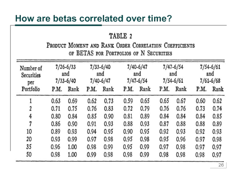
Слайд 25Is historical beta a good predictor of future beta?
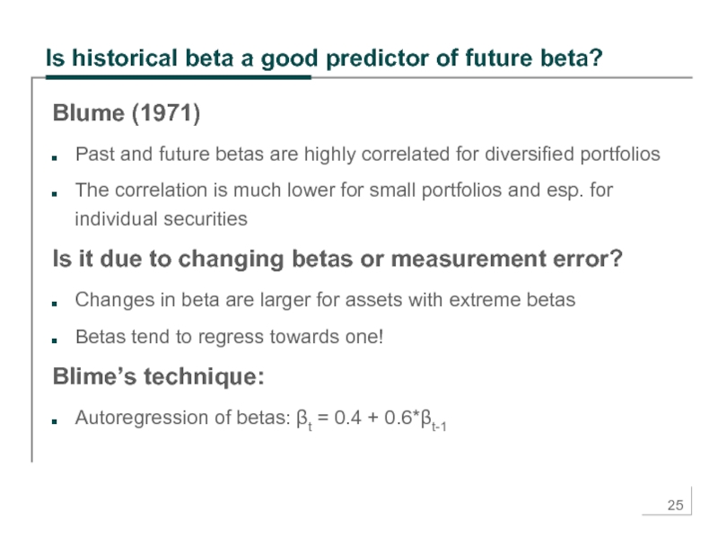
Blume (1971)
Past and
future betas are highly correlated for diversified portfolios
The correlation is much lower for small portfolios and esp. for individual securities
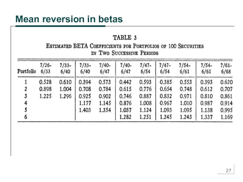
Is it due to changing betas or measurement error?
Changes in beta are larger for assets with extreme betas
Betas tend to regress towards one!
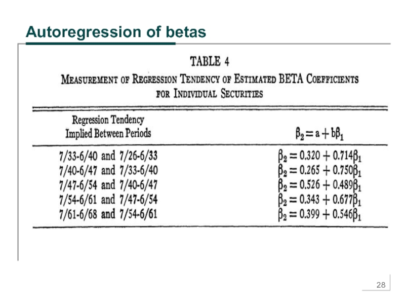
Blime’s technique:
Autoregression of betas: βt = 0.4 + 0.6*βt-1
The correlation is much lower for small portfolios and esp. for individual securities
Is it due to changing betas or measurement error?
Changes in beta are larger for assets with extreme betas
Betas tend to regress towards one!
Blime’s technique:
Autoregression of betas: βt = 0.4 + 0.6*βt-1
Слайд 29Vasicek’s adjustment
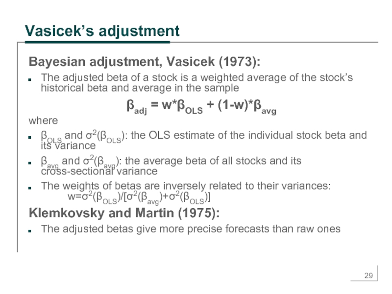
Bayesian adjustment, Vasicek (1973):
The adjusted beta of a stock is
a weighted average of the stock’s historical beta and average in the sample
βadj = w*βOLS + (1-w)*βavg
where
βOLS and σ2(βOLS): the OLS estimate of the individual stock beta and its variance
βavg and σ2(βavg): the average beta of all stocks and its cross-sectional variance
The weights of betas are inversely related to their variances: w=σ2(βOLS)/[σ2(βavg)+σ2(βOLS)]
Klemkovsky and Martin (1975):
The adjusted betas give more precise forecasts than raw ones
Слайд 30Estimating beta for illiquid stocks
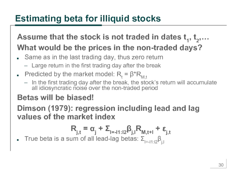
Assume that the stock is not traded
in dates t1, t2,…
What would be the prices in the non-traded days?
Same as in the last trading day, thus zero return
Large return in the first trading day after the break
Predicted by the market model: Rt = β*RM,t
In the first trading day after the break, the stock’s return will accumulate all idiosyncratic noise over the non-traded period
Betas will be biased!
Dimson (1979): regression including lead and lag values of the market index
Rj,t = αj + Σl=-l1:l2βj,lRM,t+l + εj,t
True beta is a sum of all lead-lag betas: Σl=-l1:l2βj,l
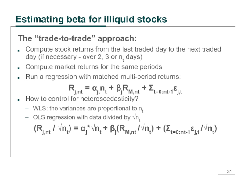
Слайд 31Estimating beta for illiquid stocks
The “trade-to-trade” approach:
Compute stock returns from
the last traded day to the next traded day (if necessary - over 2, 3 or nt days)
Compute market returns for the same periods
Run a regression with matched multi-period returns:
Rj,nt = αj,nt + βjRM,nt + Σt=0:nt-1εj,t
How to control for heteroscedasticity?
WLS: the variances are proportional to nt
OLS regression with data divided by √nt
(Rj,nt / √nt) = αj*√nt + βj(RM,nt /√nt) + (Σt=0:nt-1εj,t /√nt)
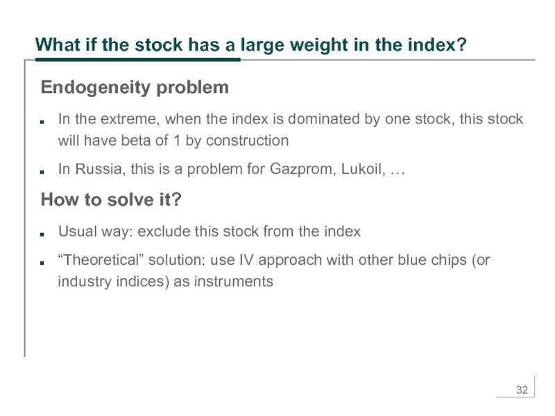
Слайд 32What if the stock has a large weight in the index?
Endogeneity
problem
In the extreme, when the index is dominated by one stock, this stock will have beta of 1 by construction
In Russia, this is a problem for Gazprom, Lukoil, …
How to solve it?
Usual way: exclude this stock from the index
“Theoretical” solution: use IV approach with other blue chips (or industry indices) as instruments
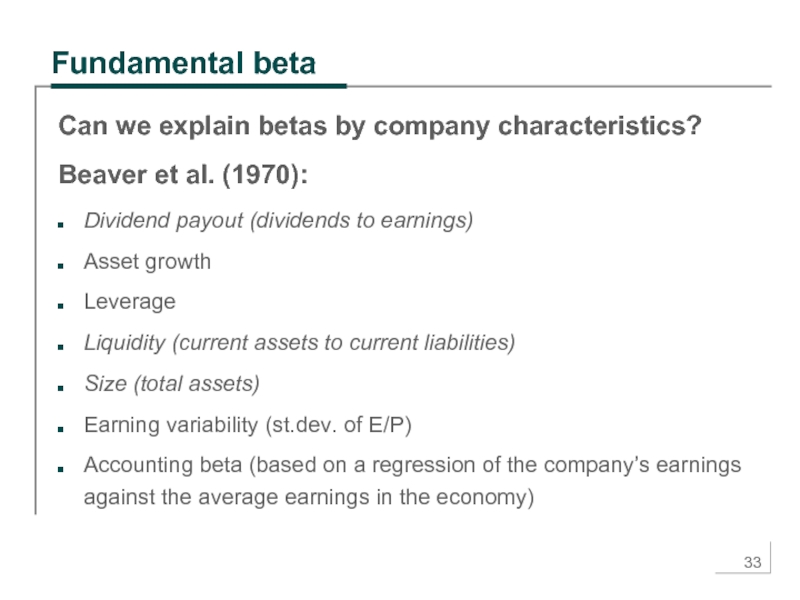
Слайд 33Fundamental beta
Can we explain betas by company characteristics?
Beaver et al. (1970):
Dividend payout (dividends to earnings)
Asset growth
Leverage
Liquidity (current assets to current liabilities)
Size (total assets)
Earning variability (st.dev. of E/P)
Accounting beta (based on a regression of the company’s earnings against the average earnings in the economy)
Слайд 34Next class
Advanced topic: testing CAPM
Is beta sufficient to describe systematic risks?
Time
series and cross-sectional tests
Market anomalies
New topic: multi-factor models
How to construct and interpret risk factors?
Most popular models: Fama-French, Carhart,…
Market anomalies
New topic: multi-factor models
How to construct and interpret risk factors?
Most popular models: Fama-French, Carhart,…

