- Главная
- Разное
- Дизайн
- Бизнес и предпринимательство
- Аналитика
- Образование
- Развлечения
- Красота и здоровье
- Финансы
- Государство
- Путешествия
- Спорт
- Недвижимость
- Армия
- Графика
- Культурология
- Еда и кулинария
- Лингвистика
- Английский язык
- Астрономия
- Алгебра
- Биология
- География
- Детские презентации
- Информатика
- История
- Литература
- Маркетинг
- Математика
- Медицина
- Менеджмент
- Музыка
- МХК
- Немецкий язык
- ОБЖ
- Обществознание
- Окружающий мир
- Педагогика
- Русский язык
- Технология
- Физика
- Философия
- Химия
- Шаблоны, картинки для презентаций
- Экология
- Экономика
- Юриспруденция
Shortest Paths презентация
Содержание
- 1. Shortest Paths
- 2. Dijkstra’s algorithm are given: source vertex s;
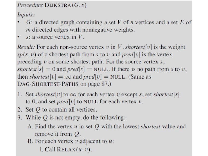
- 3. Dijkstra’s algorithm
- 4. Dijkstra’s algorithm the situation at time 0 shortest[s]= 0
- 5. Dijkstra’s algorithm at time 4 shortest[y]= 4, pred[y]= s
- 6. Dijkstra’s algorithm at time 5 shortest[t]=5, pred[t]= y
- 7. Dijkstra’s algorithm at time 7 shortest[z]=7, pred[z]= y
- 8. Dijkstra’s algorithm at time 8 shortest[x]=8, pred[x]=t
- 9. Dijkstra’s algorithm Dijkstra’s algorithm works a little
- 11. Dijkstra’s algorithm A set Q is a
- 12. Dijkstra’s algorithm A set Q is a
- 13. Dijkstra’s algorithm Question 1: How does the
- 14. Dijkstra’s algorithm
- 15. Dijkstra’s algorithm Answer to Question 1: How
- 16. Dijkstra’s algorithm Remaid: The Algorithm for Relaxing
- 17. Dijkstra’s algorithm Idea of Dijkstra’s Algorithm: Repeated
- 18. Dijkstra’s algorithm Idea of Dijkstra’s Algorithm: Repeated
- 19. Dijkstra’s algorithm Idea of Dijkstra’s Algorithm: Repeated
- 20. Dijkstra’s algorithm The Selection in Dijkstra’s Algorithm
- 21. Dijkstra’s algorithm Question 2: How does the
- 22. Dijkstra’s algorithm Question: How do we implement
- 23. Dijkstra’s algorithm Review of Priority Queues
- 24. Dijkstra’s algorithm EXTRACT-MIN (Q) removes the vertex
- 25. Dijkstra’s algorithm Example.
- 26. Dijkstra’s algorithm Step 0: Initialization. Priority Queue.
- 27. Dijkstra’s algorithm Step 1: As Adjacent[s]={a,b}, work
- 28. Dijkstra’s algorithm Step 2: After Step 1,
- 29. Dijkstra’s algorithm Step 3: After Step 2,
- 30. Dijkstra’s algorithm Step 4: After Step 3,
- 31. Dijkstra’s algorithm Step 5: After Step 4,
- 32. Dijkstra’s algorithm Shortest Path Tree: T=(V,A),
- 33. Dijkstra’s algorithm
- 34. Dijkstra’s algorithm Simple array implementation The simplest
- 35. Dijkstra’s algorithm Simple array implementation The INSERT
- 36. Dijkstra’s algorithm Simple array implementation Once we
- 37. Dijkstra’s algorithm Binary heap implementation A
- 38. Dijkstra’s algorithm
- 39. Dijkstra’s algorithm Nodes with no children, such
- 40. Dijkstra’s algorithm The node with the minimum
- 41. Dijkstra’s algorithm Therefore, we can traverse a
- 42. Dijkstra’s algorithm Fibonacci heap implementation We can

Слайд 2Dijkstra’s algorithm
are given:
source vertex s;
the weight weight (u, v) of each
edge (u, v);
to calculate:
for each vertex v the shortest-path weight sp(s, v);
=> shortest[v]
the vertex preceding v;=> pred[v]
to calculate:
for each vertex v the shortest-path weight sp(s, v);
=> shortest[v]
the vertex preceding v;=> pred[v]
 of each edge (u, v);to calculate:for")


Слайд 9Dijkstra’s algorithm
Dijkstra’s algorithm works a little differently. It treats all edges
the same.
Dijkstra’s algorithm works by calling the RELAX procedure once for each edge.
Dijkstra’s algorithm works by calling the RELAX procedure once for each edge.

Слайд 11Dijkstra’s algorithm
A set Q is a set of vertices for which
the final shortest and pred values are not yet known.
All vertices not in Q have their final shortest and pred values.
In the step 1 shortest[s] = 0, shortest[v] = ∞ for all other vertices, and pred[v] = NULL for all vertices.
All vertices not in Q have their final shortest and pred values.
In the step 1 shortest[s] = 0, shortest[v] = ∞ for all other vertices, and pred[v] = NULL for all vertices.

Слайд 12Dijkstra’s algorithm
A set Q is a set of vertices for which
the final shortest and pred values are not yet known.
All vertices not in Q have their final shortest and pred values.
In the step 1 shortest[s] = 0, shortest[v] = ∞ for all other vertices, and pred[v] = NULL for all vertices.
Algorithm repeatedly finds the vertex u in set Q with the lowest shortest value, removes that vertex from Q, and relaxes all the edges leaving u.

Слайд 13Dijkstra’s algorithm
Question 1: How does the algorithm find new paths and
do the relaxation?
Question 2: In which order does the algorithm process the vertices one by one?
Question 2: In which order does the algorithm process the vertices one by one?


Слайд 15Dijkstra’s algorithm
Answer to Question 1: How does the algorithm find new
paths and do the relaxation?
Relaxation. If the new path from s to v
is shorter than shortest[v], then update shortest[v] to the length of this new path.
Remark: Whenever we set shortest[v] to a finite value, there exists a path of that length. Therefore
shortest[v] ≥ sp(s,v).
Note: If shortest[v]= sp(s,v), then further relaxations cannot change its value.

Слайд 16Dijkstra’s algorithm
Remaid: The Algorithm for Relaxing an Edge.
Relax(u, v)
{
If (shortest[u] +
weight(u,v)< shortest[v])
{
shortest[v]= shortest[u] + weight(u,v);
pred[v]=u;
}
}
{
shortest[v]= shortest[u] + weight(u,v);
pred[v]=u;
}
}
{ If (shortest[u] + weight(u,v)< shortest[v]) { shortest[v]= shortest[u] + weight(u,v); pred[v]=u; }}")
Слайд 17Dijkstra’s algorithm
Idea of Dijkstra’s Algorithm: Repeated Relaxation
Dijkstra’s algorithm operates by maintaining
a subset of vertices, Q comprise V, for which we know the true distance, that is
shortest[v]= sp(s,v).
shortest[v]= sp(s,v).

Слайд 18Dijkstra’s algorithm
Idea of Dijkstra’s Algorithm: Repeated Relaxation
Initially Q=NULL, the empty set,
and we set shortest[s]=0 and shortest[v]=∞ for all others vertices v. One by one we select vertices from V\Q to add to Q.

Слайд 19Dijkstra’s algorithm
Idea of Dijkstra’s Algorithm: Repeated Relaxation
The set Q can be
implemented using an array of vertex colors. Initially all vertices are white, and we set color[v]=black to indicate that v comprise Q.

Слайд 20Dijkstra’s algorithm
The Selection in Dijkstra’s Algorithm
Recall Question 2: What is the
best order in which to process vertices, so that the estimates are guaranteed to converge to the true distances?
That is, how does the algorithm select which vertex among the vertices of V\Q?
That is, how does the algorithm select which vertex among the vertices of V\Q?

Слайд 21Dijkstra’s algorithm
Question 2: How does the algorithm select which vertex among
the vertices of V\Q?
Answer: We use a greedy algorithm. For each vertex in u from V\Q we have computed a distance estimate shortest[u].
The next vertex processed is always a vertex u from V\Q for which shortest[u] is minimum, that is, we take the unprocessed vertex that is closest (by our estimate) to s.
Answer: We use a greedy algorithm. For each vertex in u from V\Q we have computed a distance estimate shortest[u].
The next vertex processed is always a vertex u from V\Q for which shortest[u] is minimum, that is, we take the unprocessed vertex that is closest (by our estimate) to s.

Слайд 22Dijkstra’s algorithm
Question: How do we implement this selection of vertices efficiently?
Answer:
We store the vertices of V\Q in a priority queue, where the key value of each vertex v is shortest[v].
Note: if we implement the priority queue using a heap, we can perform the operations Insert(), Extract Min(), and Decrease Key(), each in O(logn) time.
Note: if we implement the priority queue using a heap, we can perform the operations Insert(), Extract Min(), and Decrease Key(), each in O(logn) time.

Слайд 23Dijkstra’s algorithm
Review of Priority Queues
A Priority Queue is a data structure
(can be implemented as a heap) which supports the following operations:
INSERT (Q; v) inserts vertex v into set Q.
(Dijkstra’s algorithm calls INSERT n times.)
…
INSERT (Q; v) inserts vertex v into set Q.
(Dijkstra’s algorithm calls INSERT n times.)
…

Слайд 24Dijkstra’s algorithm
EXTRACT-MIN (Q) removes the vertex in Q with the minimum
shortest value and returns this vertex to its caller.
(Dijkstra’s algorithm calls EXTRACT-MIN n times.)
DECREASE-KEY (Q; v) performs whatever bookkeeping is necessary in Q to record that shortest[v] was decreased by a call of RELAX. (Dijkstra’s algorithm calls DECREASE-KEY up to m times.)
(Dijkstra’s algorithm calls EXTRACT-MIN n times.)
DECREASE-KEY (Q; v) performs whatever bookkeeping is necessary in Q to record that shortest[v] was decreased by a call of RELAX. (Dijkstra’s algorithm calls DECREASE-KEY up to m times.)
 removes the vertex in Q with the minimum shortest value and returns")


Слайд 27Dijkstra’s algorithm
Step 1: As Adjacent[s]={a,b},
work on a and b and update
information.
Priority Queue:

Слайд 28Dijkstra’s algorithm
Step 2: After Step 1, a has the minimum key
in the priority queue. As Adjacent[a]={b,c,d},
work on b,c,d and update information.
work on b,c,d and update information.
Priority Queue:

Слайд 29Dijkstra’s algorithm
Step 3: After Step 2, b has the minimum key
in the priority queue. As Adjacent[b]={a,c},
work on a,c and update information.
work on a,c and update information.
Priority Queue:

Слайд 30Dijkstra’s algorithm
Step 4: After Step 3, c has the minimum key
in the priority queue. As Adjacent[c]={d},
work on d and update information.
work on d and update information.
Priority Queue:

Слайд 31Dijkstra’s algorithm
Step 5: After Step 4, d has the minimum key
in the priority queue. As Adjacent[d]={c},
work on c and update information.
work on c and update information.
Priority Queue: Q=0.

Слайд 32Dijkstra’s algorithm
Shortest Path Tree: T=(V,A),
where A={(pred[v],v)|v from V\{s}}.
The array pred[v]
is used to build the tree.
, where A={(pred[v],v)|v from V\{s}}.The array pred[v] is used to build")

Слайд 34Dijkstra’s algorithm
Simple array implementation
The simplest way to implement the priority queue
operations is to store the vertices in an array with n positions.
If the priority queue at the moment contains k vertices, then they are in the first k positions of the array, in no particular order.
If the priority queue at the moment contains k vertices, then they are in the first k positions of the array, in no particular order.

Слайд 35Dijkstra’s algorithm
Simple array implementation
The INSERT operation is easy: just add the
vertex to the next unused position in the array and increment the count.
DECREASE-KEY is even easier: do nothing! Both of these operations take constant time.
The EXTRACT-MIN operation takes O(n) time, however, since we have to look at all the vertices currently in the array to find the one with the lowest shortest value.
DECREASE-KEY is even easier: do nothing! Both of these operations take constant time.
The EXTRACT-MIN operation takes O(n) time, however, since we have to look at all the vertices currently in the array to find the one with the lowest shortest value.

Слайд 36Dijkstra’s algorithm
Simple array implementation
Once we find this vertex, deleting it is
easy: just move the vertex in the last position into the position of the deleted vertex and then decrement the count.
The n EXTRACT-MIN calls take O(n2) time.
Although the calls to RELAX take O(m) time, recall that m <= n2.
With this implementation of the priority queue therefore, Dijkstra’s algorithm takes O(n2) time, with the time dominated by the time spent in EXTRACT-MIN.
The n EXTRACT-MIN calls take O(n2) time.
Although the calls to RELAX take O(m) time, recall that m <= n2.
With this implementation of the priority queue therefore, Dijkstra’s algorithm takes O(n2) time, with the time dominated by the time spent in EXTRACT-MIN.

Слайд 37Dijkstra’s algorithm
Binary heap implementation
A binary heap organizes data as a binary
tree stored in an array.
A binary tree is a type of graph.
Its vertices are named nodes.
The edges are undirected.
Each node has 0, 1, or 2 nodes below it, which are its children.
A binary tree is a type of graph.
Its vertices are named nodes.
The edges are undirected.
Each node has 0, 1, or 2 nodes below it, which are its children.


Слайд 39Dijkstra’s algorithm
Nodes with no children, such as nodes 6 through 10,
are leaves.
A binary heap is a binary tree with three additional properties.
First, the tree is completely filled on all levels, but possibly the lowest, which is filled from the left up to a point.
Second, each node contains a key, shown inside each node.
Third, the key of each node is less than or equal to the keys of its children.

Слайд 40Dijkstra’s algorithm
The node with the minimum key must always be at
position 1. The children of the node at position i are at positions 2i and 2i + 1. Its parent is at position [i/2].
A binary heap has one other important characteristic: if it consists of n nodes, then its height – the number of edges from the root down to the farthest leaf – is only [lgn].
A binary heap has one other important characteristic: if it consists of n nodes, then its height – the number of edges from the root down to the farthest leaf – is only [lgn].

Слайд 41Dijkstra’s algorithm
Therefore, we can traverse a path from the root down
to a leaf, or from a leaf up to the root, in only O(lgn) time.
So, when Dijkstra’s algorithm uses the binary-heap implementation of a priority queue, it spends O(nlgn) time inserting vertices,
O(nlgn) time in EXTRACT-MIN operations, and O(mlgn) time in DECREASE-KEY operations.
So, when Dijkstra’s algorithm uses the binary-heap implementation of a priority queue, it spends O(nlgn) time inserting vertices,
O(nlgn) time in EXTRACT-MIN operations, and O(mlgn) time in DECREASE-KEY operations.

Слайд 42Dijkstra’s algorithm
Fibonacci heap implementation
We can also implement a priority queue by
a complicated data structure called a “Fibonacci heap” or “F-heap”.
With an F-heap,
the n INSERT and EXTRACT-MIN calls take a total of O(nlgn) time, and
the m DECREASE-KEY calls take a total of Θ(m) time, and so Dijkstra’s algorithm takes only O(nlgn + m) time.
With an F-heap,
the n INSERT and EXTRACT-MIN calls take a total of O(nlgn) time, and
the m DECREASE-KEY calls take a total of Θ(m) time, and so Dijkstra’s algorithm takes only O(nlgn + m) time.