- Главная
- Разное
- Дизайн
- Бизнес и предпринимательство
- Аналитика
- Образование
- Развлечения
- Красота и здоровье
- Финансы
- Государство
- Путешествия
- Спорт
- Недвижимость
- Армия
- Графика
- Культурология
- Еда и кулинария
- Лингвистика
- Английский язык
- Астрономия
- Алгебра
- Биология
- География
- Детские презентации
- Информатика
- История
- Литература
- Маркетинг
- Математика
- Медицина
- Менеджмент
- Музыка
- МХК
- Немецкий язык
- ОБЖ
- Обществознание
- Окружающий мир
- Педагогика
- Русский язык
- Технология
- Физика
- Философия
- Химия
- Шаблоны, картинки для презентаций
- Экология
- Экономика
- Юриспруденция
Object tracking using particle filter презентация
Содержание
- 1. Object tracking using particle filter
- 2. Overview Background Information Basic Particle Filter Theory
- 3. Object Tracking Tracking objects in video involves
- 4. Background In order to model accurately the
- 5. The Particle Filter Particle Filter
- 6. Mathematical Background Particle Filtering estimates the state
- 7. Mathematical Background Particle filtering assumes a Markov
- 8. Mathematical Background Est(t) = P( x t
- 9. Mathematical Background Final Result: Est(t) = p(y
- 10. Mathematical Background To implement Particle Filter we
- 11. Mathematical Background We sample from the proposal
- 12. Basic Particle Filter Theory
- 13. Basic Particle Filter Theory (Cont.) Particle
- 14. Basic Particle Filter Theory (Cont.) System
- 15. Basic Particle Filter Theory (Cont.) Given N
- 16. Basic Particle Filter Theory (Cont.) The basic
- 17. Particle Filter Algorithm Sequential importance
- 18. Particle Filter Algorithm Selection Step Multiply
- 19. Rao-Blackwellised Particle Filter RBPF is an extension
- 20. RBPF Approach RBPF models the states as
- 21. Implementation We have implemented the Particle Filter
- 22. Implementation Color Based Probabilistic Tracking These trackers
- 23. Color Based Probabilistic Tracking The combination of
- 24. Color Based Probabilistic Tracking Reference Color Window
- 25. Color Based Probabilistic Tracking State Space We
- 26. Color Based Probabilistic Tracking System Dynamics A
- 27. Color Based Probabilistic Tracking Observation yt The
- 28. Color Based Probabilistic Tracking Particle Filter Iteration
- 29. Color Based Probabilistic Tracking An step by
- 30. Color Based Probabilistic Tracking For each particle,
- 31. Color Based Probabilistic Tracking Calculate the histogram
- 32. Color Based Probabilistic Tracking Re-sampling step, where
- 33. Color Based Probabilistic Tracking Functions Used:
- 34. Color Based Probabilistic Tracking: Results
- 35. Applications Video Surveillance Gesture HCI
- 36. Future Work Automatic initialization of reference window. Multi part color window. Multi-object tracking.
- 37. References M. Isard and A. Blake. Condensation–conditional
- 38. Thank You

Слайд 2 Overview
Background Information
Basic Particle Filter Theory
Rao Blackwellised Particle Filter
Color Based Probabilistic Tracking

Слайд 3Object Tracking
Tracking objects in video involves the modeling of non-linear and
non-gaussian systems.
Non-Linear
Non-Gaussian
Non-Linear
Non-Gaussian

Слайд 4 Background
In order to model accurately the underlying dynamics of a physical
system, it is important to include elements of non-linearity and non-gaussianity in many application areas.
Particle Filters can be used to achieve this.
They are sequential Monte Carlo methods based on point mass representations of probability densities, which are applied to any state model.
Particle Filters can be used to achieve this.
They are sequential Monte Carlo methods based on point mass representations of probability densities, which are applied to any state model.

Слайд 5 The Particle Filter
Particle Filter is concerned with the problem
of tracking single and multiple objects.
Particle Filter is a hypothesis tracker, that approximates the filtered posterior distribution by a set of weighted particles.
It weights particles based on a likelihood score and then propagates these particles according to a motion model.
Particle Filter is a hypothesis tracker, that approximates the filtered posterior distribution by a set of weighted particles.
It weights particles based on a likelihood score and then propagates these particles according to a motion model.

Слайд 6Mathematical Background
Particle Filtering estimates the state of the system, x t,
as time t as the Posterior distribution:
P( x t | y 0-t )
Let,
Est (t) = P( x t | y 0-t )
Est(1) can be initialized using prior knowledge
P( x t | y 0-t )
Let,
Est (t) = P( x t | y 0-t )
Est(1) can be initialized using prior knowledge

Слайд 7Mathematical Background
Particle filtering assumes a Markov Model for system state estimation.
Markov model states that past and future states are conditionally independent given current state.
Thus, observations are dependent only on current state.

Слайд 8Mathematical Background
Est(t) = P( x t | y 0 - t
)
= p(y t | x t, y 0 – t-1).P(x t | y 0 – t-1)
(Using Baye’s Theorem)
= p(y t | x t ). P(x t | y 0 – t-1)
(Using Markov model)
= p(y t | x t ). P(x t |x t-1).P(x t-1 | y 0 – t-1)
= p(y t | x t ). P(x t |x t-1).Est(t-1)
= p(y t | x t, y 0 – t-1).P(x t | y 0 – t-1)
(Using Baye’s Theorem)
= p(y t | x t ). P(x t | y 0 – t-1)
(Using Markov model)
= p(y t | x t ). P(x t |x t-1).P(x t-1 | y 0 – t-1)
= p(y t | x t ). P(x t |x t-1).Est(t-1)
 = P( x t | y 0 - t ) = p(y t")
Слайд 9Mathematical Background
Final Result:
Est(t) = p(y t | x t ). P(x
t |x t-1).Est(t-1)
Where:
p(y t | x t ): Observation Model
P(x t |x t-1).Est(t-1): Proposal distribution
Where:
p(y t | x t ): Observation Model
P(x t |x t-1).Est(t-1): Proposal distribution
 = p(y t | x t ). P(x t |x t-1).Est(t-1) Where:p(y t")
Слайд 10Mathematical Background
To implement Particle Filter we need
State Motion model: P(x t
|x t-1)
Observation Model: p(y t | x t ):
Initial State: Est(1)
Observation Model: p(y t | x t ):
Initial State: Est(1)
Observation Model: p(y")
Слайд 11Mathematical Background
We sample from the proposal and not the posterior for
estimation.
To take into account that we will be sampling from wrong distribution, the samples have to be likelihood weighed by ratio of posterior and proposal distribution:
W t = Posterior i.e.Est (t) / proposal Distribution
= p(y t | x t )
Thus, weight of particle should be changed depending on observation for current frame.

Слайд 12 Basic Particle Filter Theory
A discrete set of samples or
particles represents the object-state and evolves over time driven by the means of "survival of the fittest". Nonlinear motion models can be used to predict object-states.

Слайд 13Basic Particle Filter Theory (Cont.)
Particle Filter is concerned with the
estimation of the distribution of a stochastic process at any time instant, given some partial information up to that time.
The basic model usually consists of a Markov chain X and a possibly nonlinear observation Y with observational noise V independent of the signal X.
The basic model usually consists of a Markov chain X and a possibly nonlinear observation Y with observational noise V independent of the signal X.
Particle Filter is concerned with the estimation of the distribution of")
Слайд 14Basic Particle Filter Theory (Cont.)
System Dynamics ie.Motion Model:
p(x t| x
0:t-1)
Observation Model:
p(y t | x t)
Posterior Distribution:
p(x t | y o..t)
Proposal Distribution is the Motion Model
Weight, w t = Posterior / Proposal = observation
Observation Model:
p(y t | x t)
Posterior Distribution:
p(x t | y o..t)
Proposal Distribution is the Motion Model
Weight, w t = Posterior / Proposal = observation
System Dynamics ie.Motion Model: p(x t| x 0:t-1)Observation Model: p(y t | x")
Слайд 15Basic Particle Filter Theory (Cont.)
Given N particles (samples)
{x(i)0:t-1,z(i)0:t-1}Ni=1 at time t-1, approximately distributed according to the distribution P(dx(i)0:t-1,z(i)0:t-1|y1:t-1), particle filters enable us to compute N particles {x(i)0:t,z(i)0:t}Ni=1 approximately distributed according to the posterior distribution P(dx(i)0:t,z(i)0:t|y1:t)
Given N particles (samples) {x(i)0:t-1,z(i)0:t-1}Ni=1 at")
Слайд 16Basic Particle Filter Theory (Cont.)
The basic Particle Filter algorithm consists of
2 steps:
Sequential importance sampling step
Selection step
Sequential importance sampling step
Selection step
The basic Particle Filter algorithm consists of 2 steps:Sequential importance sampling")
Слайд 17 Particle Filter Algorithm
Sequential importance sampling
Uses Sequential Monte Carlo simulation.
For
each particle at time t, we sample from the transition priors
For each particle we then evaluate and normalize the importance weights.
For each particle we then evaluate and normalize the importance weights.

Слайд 18 Particle Filter Algorithm
Selection Step
Multiply or discard particles with respect to
high or low importance weights w(i)t to obtain N particles.
This selection step is what allows us to track moving objects efficiently.
This selection step is what allows us to track moving objects efficiently.

Слайд 19Rao-Blackwellised Particle Filter
RBPF is an extension on PF.
It uses PF to
compute the distribution of discrete state with Kalman Filter to compute the distribution of continuous state.
For each sample of the discrete states, the mean and covariance of the continuous state are updated using the exact computations.
We have implemented the particle filter algorithm and not the RBPF.
For each sample of the discrete states, the mean and covariance of the continuous state are updated using the exact computations.
We have implemented the particle filter algorithm and not the RBPF.

Слайд 20 RBPF Approach
RBPF models the states as
Ct is the continuous state
representation
Dt is the discrete state representation
The aim of this approach is to predict the discrete state Dt.
However, for our object tracking application, the above approach was unsuitable.
Dt is the discrete state representation
The aim of this approach is to predict the discrete state Dt.
However, for our object tracking application, the above approach was unsuitable.

Слайд 21 Implementation
We have implemented the Particle Filter algorithm in Matlab.
Our approach towards
this project:
Reading research papers on PF given to us by Dr.Latecki.
Trying to implement PF-RBPF algorithm written by Nando de Freitas.
Reading research papers on PF given to us by Dr.Latecki.
Trying to implement PF-RBPF algorithm written by Nando de Freitas.

Слайд 22 Implementation
Color Based Probabilistic Tracking
These trackers rely on the deterministic search
of a window, whose color content matches a reference histogram color model.
Uses principle of color histogram distance.
This color based tracking is very flexible and can be extended in many ways.
Uses principle of color histogram distance.
This color based tracking is very flexible and can be extended in many ways.

Слайд 23Color Based Probabilistic Tracking
The combination of tools used to accomplish a
given tracking task depends on whether one tries to track:
Objects of a given nature eg.cars,faces
Objects of a given nature with a specific attribute eg.moving cars, face of specific person
Objects of unknown nature, but of specific interest to us eg.moving objects.
Objects of a given nature eg.cars,faces
Objects of a given nature with a specific attribute eg.moving cars, face of specific person
Objects of unknown nature, but of specific interest to us eg.moving objects.

Слайд 24Color Based Probabilistic Tracking
Reference Color Window
The target object to be tracked
forms the reference color window.
Its histogram is calculated, which is used to compute the histogram distance while performing a deterministic search for a matching window.
Its histogram is calculated, which is used to compute the histogram distance while performing a deterministic search for a matching window.

Слайд 25Color Based Probabilistic Tracking
State Space
We have modeled the states, as its
location in each frame of the video.
The state space is represented in the spatial domain as:
X = ( x , y )
We have initialized the state space for the first frame manually.
The state space is represented in the spatial domain as:
X = ( x , y )
We have initialized the state space for the first frame manually.

Слайд 26Color Based Probabilistic Tracking
System Dynamics
A second-order auto-regressive dynamics is chosen on
the parameters used to represent our state space i.e (x,y).
The dynamics is given as:
Xt+1 = Axt + Bxt-1
Matrices A and B could be learned from a set of sequences where correct tracks have been obtained.
We have used an ad-hoc model for our implementation.
The dynamics is given as:
Xt+1 = Axt + Bxt-1
Matrices A and B could be learned from a set of sequences where correct tracks have been obtained.
We have used an ad-hoc model for our implementation.

Слайд 27Color Based Probabilistic Tracking
Observation yt
The observation yt is proportional to the
histogram distance between the color window of the predicted location in the frame and the reference color window.
Yt α Dist(q,qx),
Where
q = reference color histogram.
qx = color histogram of predicted location.
Yt α Dist(q,qx),
Where
q = reference color histogram.
qx = color histogram of predicted location.

Слайд 28Color Based Probabilistic Tracking
Particle Filter Iteration
Steps:
Initialize xt for first frame
Generate
a particle set of N particles {xmt}m=1..N
Prediction for each particle using second order auto-regressive dynamics.
Compute histogram distance
Weigh each particle based on histogram distance
Select the location of target as a particle with minimum histogram distance.
Sampling the particles for next iteration.
Prediction for each particle using second order auto-regressive dynamics.
Compute histogram distance
Weigh each particle based on histogram distance
Select the location of target as a particle with minimum histogram distance.
Sampling the particles for next iteration.

Слайд 29Color Based Probabilistic Tracking
An step by step look at our code,
highlighting the concepts applied:
Initialization of state space for the first frame and calculating the reference histogram:
reference = imread('reference.jpg');
[ref_count,ref_bin] = imhist(reference);
x1= 45; y1= 45;
Describing the N particles within a specified window:
for i = 1:N
x(1,i,1) = x1 + 50 * rand(1) - 50 *rand(1);
x(2,i,1) = y1 + 50 * rand(1) - 50 *rand(1);
end

Слайд 30Color Based Probabilistic Tracking
For each particle, we apply the second order
dynamics equation to predict new states:
if (j==2) x(:,i,j) = A * x(:,i,j-1);
else x(:,i,j)=rand(n_x)*x(:,i,j-1)+rand(n_x)*x(:,i,j-2);
The color window is defined and the histogram is calculated:
rect = [(x(1,i,j)-15),(x(2,i,j)-15),30,30];
[count,binnumber] = imhist(imcrop(I(:,:,:,j),rect));
if (j==2) x(:,i,j) = A * x(:,i,j-1);
else x(:,i,j)=rand(n_x)*x(:,i,j-1)+rand(n_x)*x(:,i,j-2);
The color window is defined and the histogram is calculated:
rect = [(x(1,i,j)-15),(x(2,i,j)-15),30,30];
[count,binnumber] = imhist(imcrop(I(:,:,:,j),rect));

Слайд 31Color Based Probabilistic Tracking
Calculate the histogram distance:
for k = 1:255
d( I
, j ) = d( i, j ) + (double ( count ( k ) ) - double(ref_count( k ) ) ) ^ 2;
end
Calculating the normalized weight for each particle:
w(:,j) = w(:,j)./sum(w(:,j));
w(:,j) = one(:,1) - w(:,j);
end
Calculating the normalized weight for each particle:
w(:,j) = w(:,j)./sum(w(:,j));
w(:,j) = one(:,1) - w(:,j);
 =")
Слайд 32Color Based Probabilistic Tracking
Re-sampling step, where the new particle set is
chosen:
for i = 1:N
x(1,i,j) = state(1,j) + 50 * rand(1) - 50 *rand(1);
x(2,i,j) = state(2,j) + 50 * rand(1) - 50 *rand(1);
end
for i = 1:N
x(1,i,j) = state(1,j) + 50 * rand(1) - 50 *rand(1);
x(2,i,j) = state(2,j) + 50 * rand(1) - 50 *rand(1);
end

Слайд 33Color Based Probabilistic Tracking
Functions Used:
Track_final1.m : PF tracking code
multinomialR.m : Resampling
function.


Слайд 35 Applications
Video Surveillance
Gesture HCI
Reality and Visual Effects
Medical Imaging
State estimation of
Rovers in outer-space.

Слайд 36 Future Work
Automatic initialization of reference window.
Multi part color window.
Multi-object tracking.

Слайд 37 References
M. Isard and A. Blake. Condensation–conditional density propagation for visual tracking.
Int. J. Computer Vision, 29(1):5–28, 1998.
D. Reid, “An algorithm for tracking multiple targets,” IEEE Trans. on Automation and Control, vol. AC-24,pp. 84–90, December 1979.
N. Gordon, D. Salmond, and A. Smith, “Novel approach to nonlinear/non-Gaussian Bayesian state estimation,” IEEE Procedings F, vol. 140, no. 2, pp. 107–113, 1993.
S. Arulampalam, S. Maskell, N. Gordon, and T. Clapp, “A tutorial on particle filters for on-line non-linear/non-Gaussian Bayesian tracking,” IEEE Transactions on Signal Processing, vol. 50, pp. 174–188, Feb. 2002.