of 105
- Главная
- Разное
- Дизайн
- Бизнес и предпринимательство
- Аналитика
- Образование
- Развлечения
- Красота и здоровье
- Финансы
- Государство
- Путешествия
- Спорт
- Недвижимость
- Армия
- Графика
- Культурология
- Еда и кулинария
- Лингвистика
- Английский язык
- Астрономия
- Алгебра
- Биология
- География
- Детские презентации
- Информатика
- История
- Литература
- Маркетинг
- Математика
- Медицина
- Менеджмент
- Музыка
- МХК
- Немецкий язык
- ОБЖ
- Обществознание
- Окружающий мир
- Педагогика
- Русский язык
- Технология
- Физика
- Философия
- Химия
- Шаблоны, картинки для презентаций
- Экология
- Экономика
- Юриспруденция
Introduction to normal distributions презентация
Содержание
- 1. Introduction to normal distributions
- 2. Section 6-1 Objectives Interpret graphs of normal
- 3. Properties of Normal Distributions Normal distribution
- 4. Properties of Normal Distributions The mean, median,
- 5. Properties of Normal Distributions Between μ –
- 6. Means and Standard Deviations A normal distribution
- 7. Example: Understanding Mean and Standard Deviation Which
- 8. Example: Understanding Mean and Standard Deviation Which
- 9. Example: Interpreting Graphs The scaled test scores
- 10. The Standard Normal Distribution Standard normal distribution
- 11. The Standard Normal Distribution If each data
- 12. Properties of the Standard Normal Distribution The
- 13. Properties of the Standard Normal Distribution The
- 14. Example: Using The Standard Normal Table Find
- 15. Example: Using The Standard Normal Table Find
- 16. Finding Areas Under the Standard Normal Curve
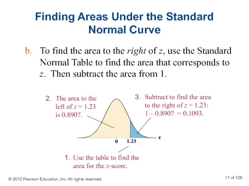
- 17. Finding Areas Under the Standard Normal Curve
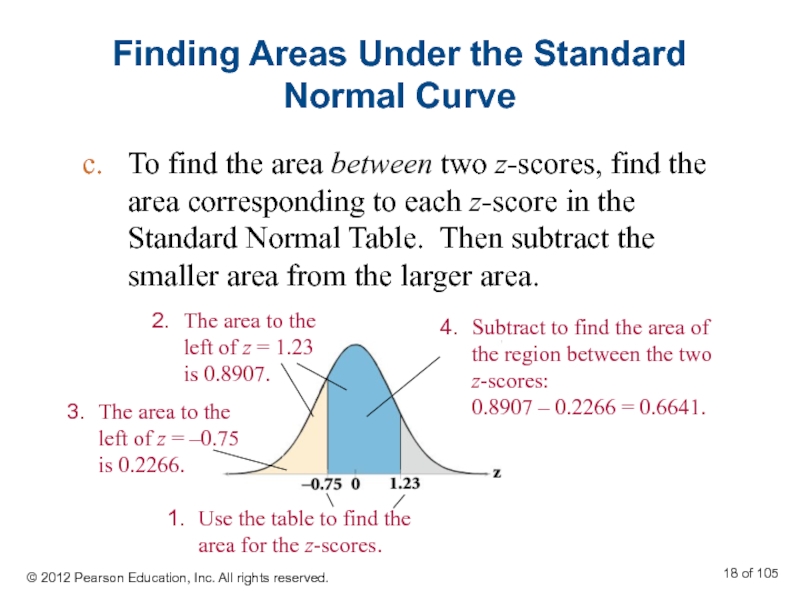
- 18. Finding Areas Under the Standard Normal Curve
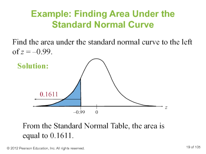
- 19. Example: Finding Area Under the Standard
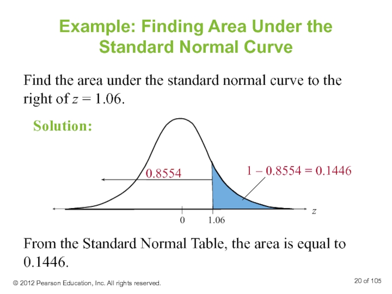
- 20. Example: Finding Area Under the Standard Normal
- 21. Find the area under the standard normal
Слайд 1Section 6-1
Introduction to Normal Distributions
© 2012 Pearson Education, Inc. All rights
Слайд 2Section 6-1 Objectives
Interpret graphs of normal probability distributions
Find areas under the
© 2012 Pearson Education, Inc. All rights reserved.
of 105
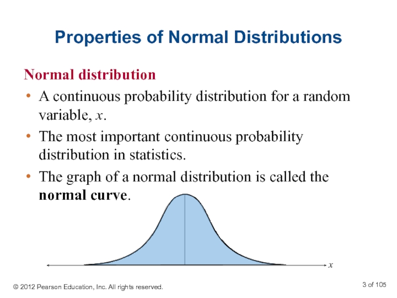
Слайд 3Properties of Normal Distributions
Normal distribution
A continuous probability distribution for a
The most important continuous probability distribution in statistics.
The graph of a normal distribution is called the normal curve.
© 2012 Pearson Education, Inc. All rights reserved.
of 105
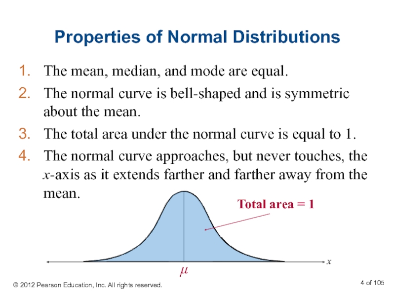
Слайд 4Properties of Normal Distributions
The mean, median, and mode are equal.
The normal
The total area under the normal curve is equal to 1.
The normal curve approaches, but never touches, the x-axis as it extends farther and farther away from the mean.
μ
© 2012 Pearson Education, Inc. All rights reserved.
of 105
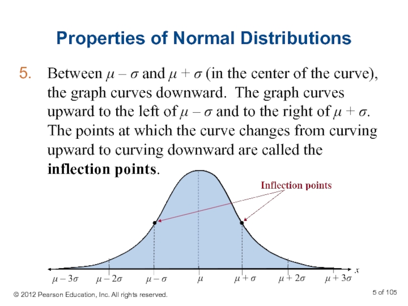
Слайд 5Properties of Normal Distributions
Between μ – σ and μ + σ
© 2012 Pearson Education, Inc. All rights reserved.
of 105
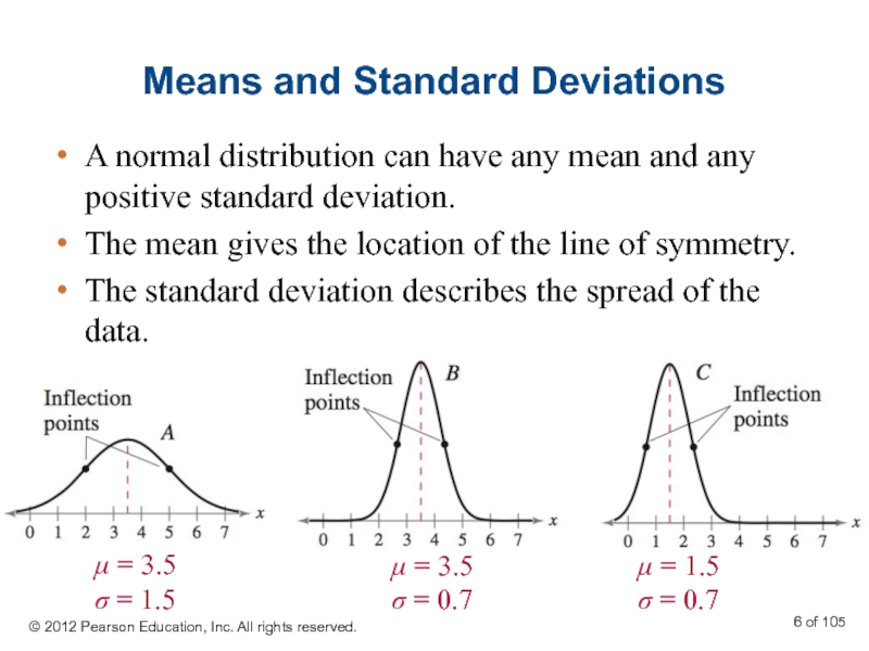
Слайд 6Means and Standard Deviations
A normal distribution can have any mean and
The mean gives the location of the line of symmetry.
The standard deviation describes the spread of the data.
© 2012 Pearson Education, Inc. All rights reserved.
of 105
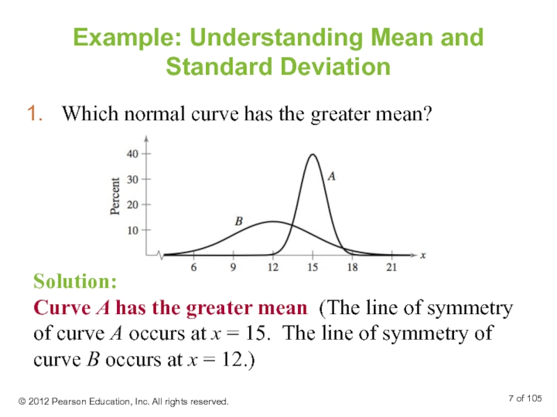
Слайд 7Example: Understanding Mean and Standard Deviation
Which normal curve has the greater
Solution:
Curve A has the greater mean (The line of symmetry of curve A occurs at x = 15. The line of symmetry of curve B occurs at x = 12.)
© 2012 Pearson Education, Inc. All rights reserved.
of 105
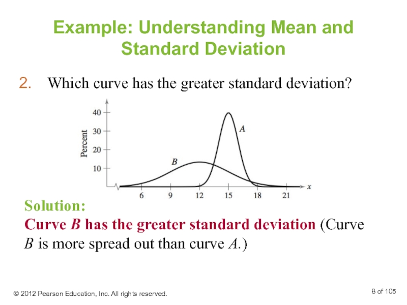
Слайд 8Example: Understanding Mean and Standard Deviation
Which curve has the greater standard
Solution:
Curve B has the greater standard deviation (Curve B is more spread out than curve A.)
© 2012 Pearson Education, Inc. All rights reserved.
of 105
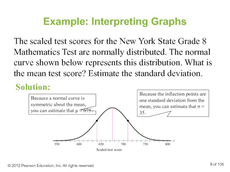
Слайд 9Example: Interpreting Graphs
The scaled test scores for the New York State
Solution:
© 2012 Pearson Education, Inc. All rights reserved.
of 105
Because a normal curve is symmetric about the mean, you can estimate that μ ≈ 675.
Because the inflection points are one standard deviation from the mean, you can estimate that σ ≈ 35.
Слайд 10The Standard Normal Distribution
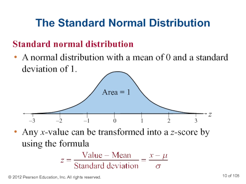
Standard normal distribution
A normal distribution with a
Any x-value can be transformed into a z-score by using the formula
© 2012 Pearson Education, Inc. All rights reserved.
of 105
Слайд 11The Standard Normal Distribution
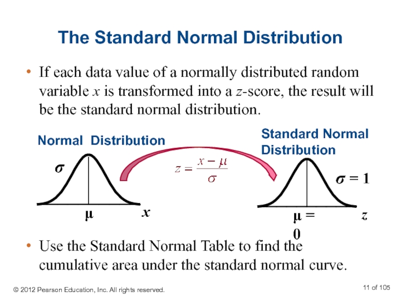
If each data value of a normally distributed
Use the Standard Normal Table to find the cumulative area under the standard normal curve.
© 2012 Pearson Education, Inc. All rights reserved.
of 105
Слайд 12Properties of the Standard Normal Distribution
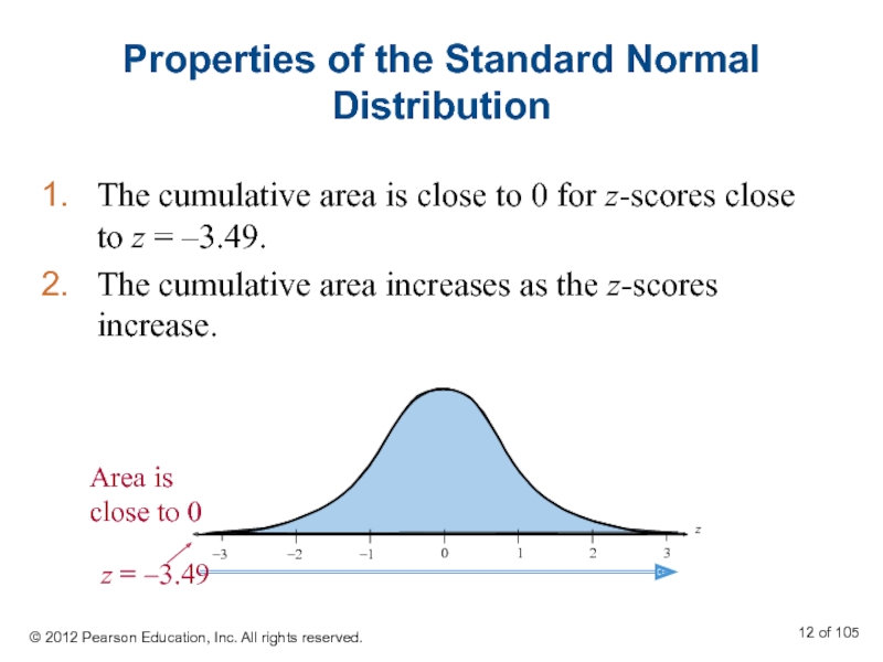
The cumulative area is close to
The cumulative area increases as the z-scores increase.
© 2012 Pearson Education, Inc. All rights reserved.
of 105
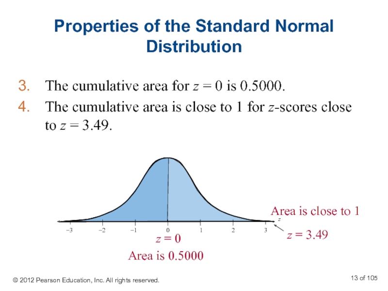
Слайд 13Properties of the Standard Normal Distribution
The cumulative area for z =
The cumulative area is close to 1 for z-scores close to z = 3.49.
© 2012 Pearson Education, Inc. All rights reserved.
of 105
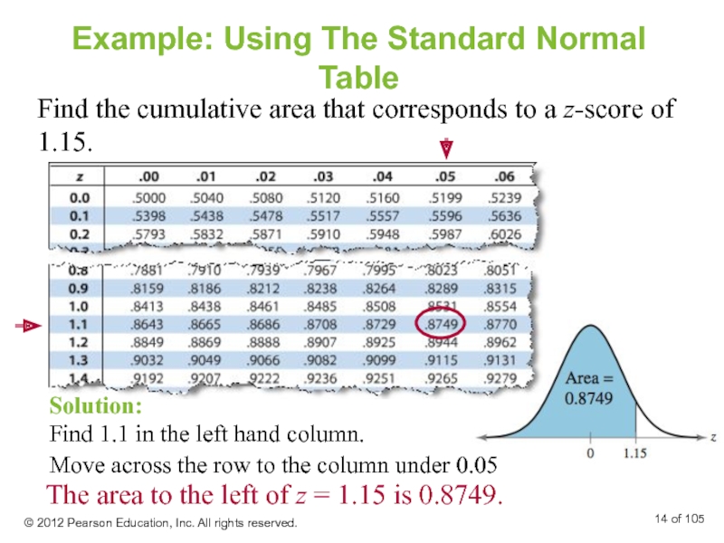
Слайд 14Example: Using The Standard Normal Table
Find the cumulative area that corresponds
The area to the left of z = 1.15 is 0.8749.
Move across the row to the column under 0.05
Solution:
Find 1.1 in the left hand column.
© 2012 Pearson Education, Inc. All rights reserved.
of 105
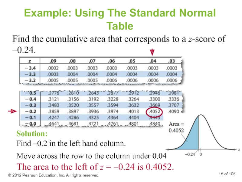
Слайд 15Example: Using The Standard Normal Table
Find the cumulative area that corresponds
Solution:
Find –0.2 in the left hand column.
The area to the left of z = –0.24 is 0.4052.
© 2012 Pearson Education, Inc. All rights reserved.
of 105
Move across the row to the column under 0.04
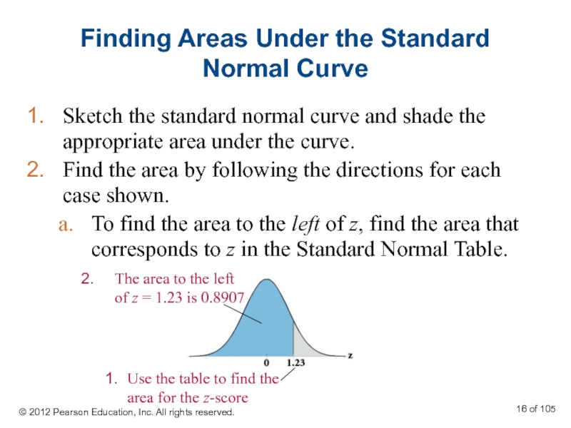
Слайд 16Finding Areas Under the Standard Normal Curve
Sketch the standard normal curve
Find the area by following the directions for each case shown.
To find the area to the left of z, find the area that corresponds to z in the Standard Normal Table.
© 2012 Pearson Education, Inc. All rights reserved.
of 105
Слайд 17Finding Areas Under the Standard Normal Curve
To find the area to
© 2012 Pearson Education, Inc. All rights reserved.
of 105
Слайд 18Finding Areas Under the Standard Normal Curve
To find the area between
© 2012 Pearson Education, Inc. All rights reserved.
of 105
Слайд 19
Example: Finding Area Under the Standard Normal Curve
Find the area under
From the Standard Normal Table, the area is equal to 0.1611.
Solution:
© 2012 Pearson Education, Inc. All rights reserved.
of 105
Слайд 20Example: Finding Area Under the Standard Normal Curve
Find the area under
From the Standard Normal Table, the area is equal to 0.1446.
Solution:
© 2012 Pearson Education, Inc. All rights reserved.
of 105
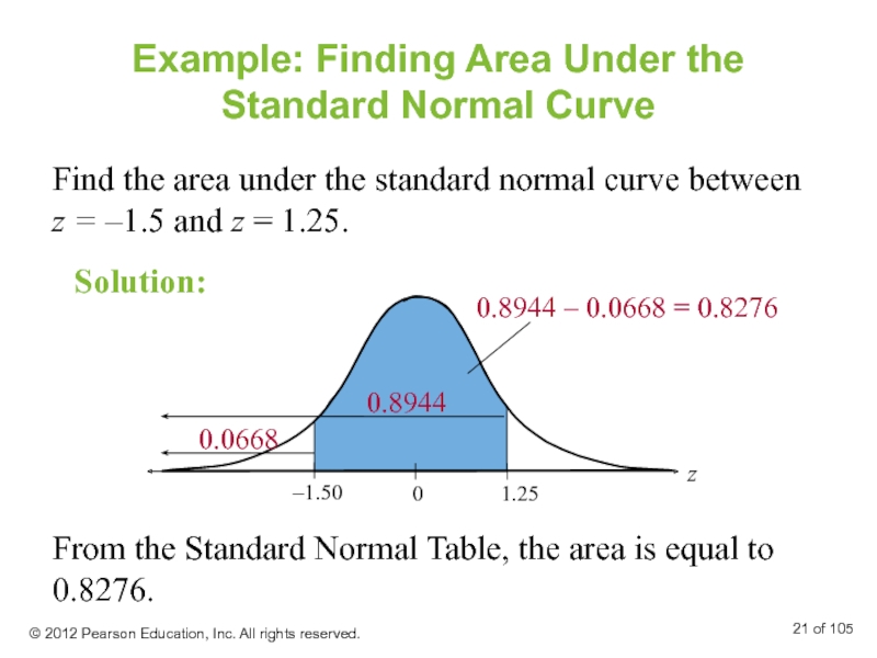
Слайд 21Find the area under the standard normal curve between z =
Example: Finding Area Under the Standard Normal Curve
From the Standard Normal Table, the area is equal to 0.8276.
Solution:
© 2012 Pearson Education, Inc. All rights reserved.
of 105
