is not related to the sample selected from the second population. The two samples are dependent if each member of one sample corresponds to a member of the other sample. Dependent samples are also called paired samples or matched samples.
- Главная
- Разное
- Дизайн
- Бизнес и предпринимательство
- Аналитика
- Образование
- Развлечения
- Красота и здоровье
- Финансы
- Государство
- Путешествия
- Спорт
- Недвижимость
- Армия
- Графика
- Культурология
- Еда и кулинария
- Лингвистика
- Английский язык
- Астрономия
- Алгебра
- Биология
- География
- Детские презентации
- Информатика
- История
- Литература
- Маркетинг
- Математика
- Медицина
- Менеджмент
- Музыка
- МХК
- Немецкий язык
- ОБЖ
- Обществознание
- Окружающий мир
- Педагогика
- Русский язык
- Технология
- Физика
- Философия
- Химия
- Шаблоны, картинки для презентаций
- Экология
- Экономика
- Юриспруденция
Definition. Statistics презентация
Содержание
- 1. Definition. Statistics
- 2. Ex. 1a: Independent and Dependent Samples Classify
- 3. Ex. 1: Independent and Dependent Samples Sample
- 4. Ex. 1b: Independent and Dependent Samples Classify
- 5. Ex. 1b: Independent and Dependent Samples Sample
- 6. Note: Dependent samples often involve identical twins,
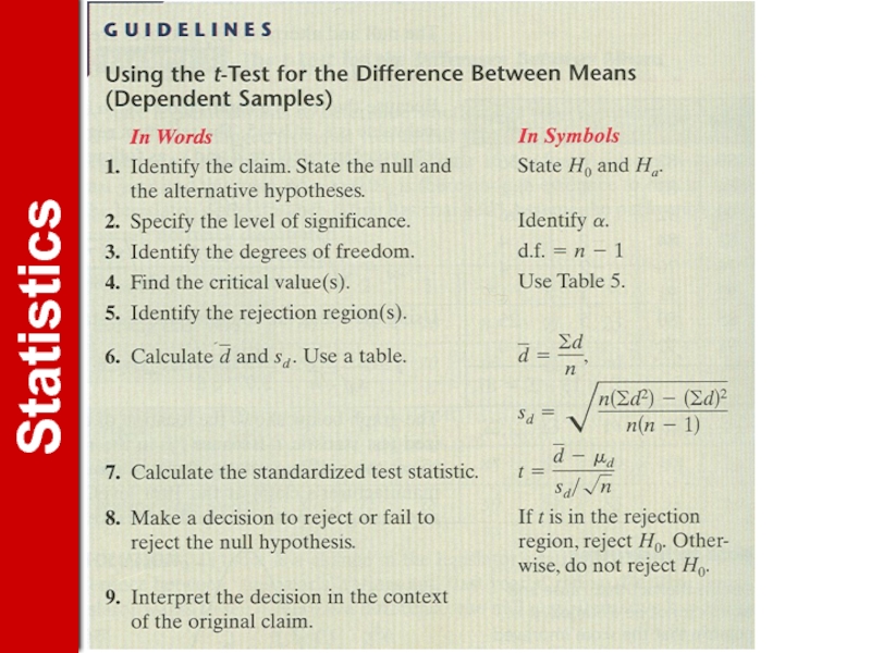
- 7. The t-Test for the Difference Between Means
- 8. To conduct the test, the following conditions
- 9. To conduct the test, the following conditions
- 10. The following symbols are used for the
- 11. Because the sampling distribution for
- 13. Ex. 2: The t-Test for the Difference
- 14. The claim is that “golfers can lower
- 15. Because the test is a right-tailed test,
- 16. Using the t-test, the standardized test statistic
- 17. Ex. 3: The t-Test for the Difference
- 18. If there is a change in the
- 19. Because the test is a tw0-tailed test,
- 20. Using the t-test, the standardized test statistic
- 21. Using Technology If you prefer to use
- 22. Using Technology Stat|Edit|enter data Subtract L1 –

Слайд 2Ex. 1a: Independent and Dependent Samples
Classify each pair of samples as
independent or dependent:
Sample 1: Resting heart rates of 35 individuals before drinking coffee.
Sample 2: Resting heart rates of the same individuals after drinking two cups of coffee.
Sample 1: Resting heart rates of 35 individuals before drinking coffee.
Sample 2: Resting heart rates of the same individuals after drinking two cups of coffee.

Слайд 3Ex. 1: Independent and Dependent Samples
Sample 1: Resting heart rates of
35 individuals before drinking coffee.
Sample 2: Resting heart rates of the same individuals after drinking two cups of coffee.
These samples are dependent. Because the resting heart rates of the same individuals were taken, the samples are related. The samples can be paired with respect to each individual.
Sample 2: Resting heart rates of the same individuals after drinking two cups of coffee.
These samples are dependent. Because the resting heart rates of the same individuals were taken, the samples are related. The samples can be paired with respect to each individual.

Слайд 4Ex. 1b: Independent and Dependent Samples
Classify each pair of samples as
independent or dependent:
Sample 1: Test scores for 35 statistics students
Sample 2: Test scores for 42 biology students who do not study statistics
Sample 1: Test scores for 35 statistics students
Sample 2: Test scores for 42 biology students who do not study statistics

Слайд 5Ex. 1b: Independent and Dependent Samples
Sample 1: Test scores for 35
statistics students
Sample 2: Test scores for 42 biology students who do not study statistics
These samples are independent. It is not possible to form a pairing between the members of samples—the sample sizes are different and the data represent test scores for different individuals.
Sample 2: Test scores for 42 biology students who do not study statistics
These samples are independent. It is not possible to form a pairing between the members of samples—the sample sizes are different and the data represent test scores for different individuals.

Слайд 6Note:
Dependent samples often involve identical twins, before and after results for
the same person or object, or results of individuals matched for specific characteristics.

Слайд 7The t-Test for the Difference Between Means
To perform a two-sample hypothesis
test with dependent samples, you will use a different technique. You will first find the difference for each data pair,
. The test statistic is the mean of these differences,
. The test statistic is the mean of these differences,

Слайд 8To conduct the test, the following conditions are required:
The samples must
be dependent (paired) and randomly selected.
Both populations must be normally distributed.
If these two requirements are met, then the sampling distribution for , the mean of the differences of the paired data entries in the dependent samples,
Both populations must be normally distributed.
If these two requirements are met, then the sampling distribution for , the mean of the differences of the paired data entries in the dependent samples,
 and")
Слайд 9To conduct the test, the following conditions are required:
has a
t-distribution with n – 1 degrees of freedom, where n is the number of data pairs.

Слайд 10The following symbols are used for the t-test for μd.
Although formulas
are given for the mean and standard deviation of differences, we suggest you use a technology tool to calculate these statistics.

Слайд 11Because the sampling distribution for is a t-distribution, you
can use a t-test to test a claim about the mean of the differences for a population of paired data.
STUDY TIP: If n > 29, use the last row (∞) in the t-distribution table.

Слайд 13Ex. 2: The t-Test for the Difference Between Means
A golf club
manufacturer claims that golfers can lower their score by using the manufacturer’s newly designed golf clubs. Eight golfers are randomly selected and each is asked to give his or her most recent score. After using the new clubs for one month, the golfers are again asked to give their most recent scores. The scores for each golfer are given in the next slide. Assuming the golf scores are normally distributed, is there enough evidence to support the manufacturer’s claim at α = 0.10?

Слайд 14The claim is that “golfers can lower their scores.” In other
words, the manufacturer claims that the score using the old clubs will be greater than the score using the new clubs. Each difference is given by:
d = (old score) – (new score)
The null and alternative hypotheses are
Ho: μd ≤ 0 and Ha: μd > 0 (claim)
d = (old score) – (new score)
The null and alternative hypotheses are
Ho: μd ≤ 0 and Ha: μd > 0 (claim)

Слайд 15Because the test is a right-tailed test, α = 0.10, and
d.f. = 8 – 1 = 7, the critical value for t is 1.415. The rejection region is t > 1.415. Using the table below, you can calculate and sd as follows:

Слайд 16Using the t-test, the standardized test statistic is:
The graph below shows
the location of the rejection region and the standardized test statistic, t. Because t is in the rejection region, you should decide to reject the null hypothesis. There is not enough evidence to support the golf manufacturer’s claim at the 10% level The results of this test indicate that after using the new clubs, golf scores were significantly lower.

Слайд 17Ex. 3: The t-Test for the Difference Between Means
A state legislator
wants to determine whether her voter’s performance rating (0-100) has changed from last year to this year. The following table shows the legislator’s performance rating for the same 16 randomly selected voters for last year and this year. At α = 0.01, is there enough evidence to conclude that the legislator’s performance rating has changed? Assume the performance ratings are normally distributed.

Слайд 18If there is a change in the legislator’s rating, there will
be a difference between “this year’s” ratings and “last year’s) ratings. Because the legislator wants to see if there is a difference, the null and alternative hypotheses are:
Ho: μd = 0 and Ha: μd ≠ 0 (claim)
Ho: μd = 0 and Ha: μd ≠ 0 (claim)

Слайд 19Because the test is a tw0-tailed test, α = 0.01, and
d.f. = 16 – 1 = 15, the critical values for t are 2.947. The rejection region are t < -2.947 and t > 2.947.

Слайд 20Using the t-test, the standardized test statistic is:
The graph shows the
location of the rejection region and the standardized test statistic, t. Because t is not in the rejection region, you should fail to reject the null hypothesis at the 1% level. There is not enough evidence to conclude that the legislator’s approval rating has changed.

Слайд 21Using Technology
If you prefer to use a technology tool for this
type of test, enter the data in two columns and form a third column in which you calculate the difference for each pair. You can now perform a one-sample t-test on the difference column as shown in Chapter 7.
Stat|Edit|enter data
Subtract L1 – L2 = in L3.
STAT|Tests|t-test
Data
μ = 0
List: L3
Freq: 1
μ ≠ 0
Calculate

Слайд 22Using Technology
Stat|Edit|enter data
Subtract L1 – L2 = in L3.
STAT|Tests|t-test
Data
μ = 0
List: L3
Freq: 1
μ ≠ 0
Calculate
μ ≠ 0
T = 1.369 (standardized test statistic)
P = don’t worry about it
X bar = 3.3125 – same as d bar.
Sx = 9.68 which is Sd
I find it easy to draw and enter the data into the curve part so I can visually see the rejection region. You will need to answer “reject” or “fail to reject” and answer whether or not there is enough evidence at whatever level given.