- Главная
- Разное
- Дизайн
- Бизнес и предпринимательство
- Аналитика
- Образование
- Развлечения
- Красота и здоровье
- Финансы
- Государство
- Путешествия
- Спорт
- Недвижимость
- Армия
- Графика
- Культурология
- Еда и кулинария
- Лингвистика
- Английский язык
- Астрономия
- Алгебра
- Биология
- География
- Детские презентации
- Информатика
- История
- Литература
- Маркетинг
- Математика
- Медицина
- Менеджмент
- Музыка
- МХК
- Немецкий язык
- ОБЖ
- Обществознание
- Окружающий мир
- Педагогика
- Русский язык
- Технология
- Физика
- Философия
- Химия
- Шаблоны, картинки для презентаций
- Экология
- Экономика
- Юриспруденция
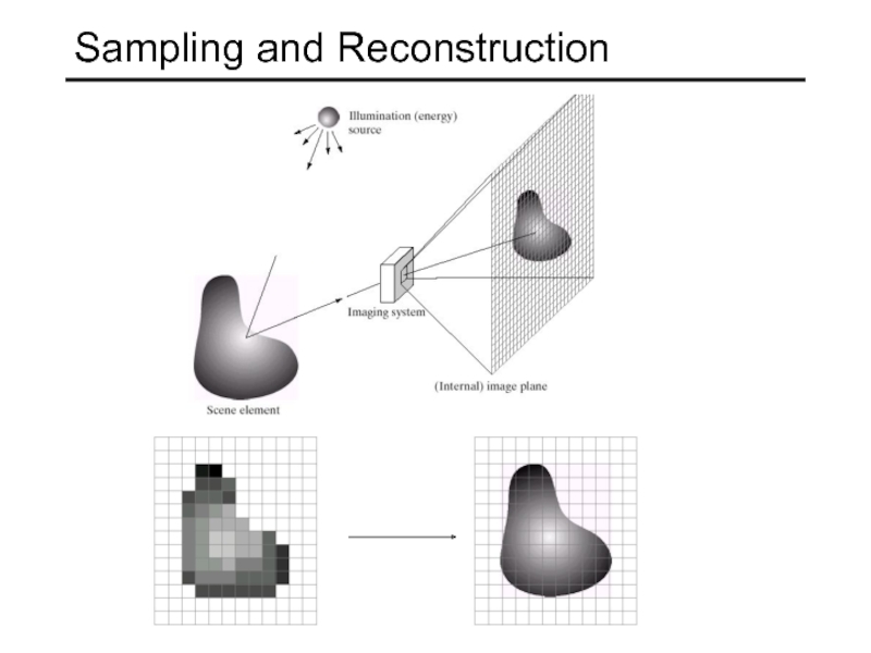
Sampling and Reconstruction презентация
Содержание
- 1. Sampling and Reconstruction
- 2. Sampling and Reconstruction
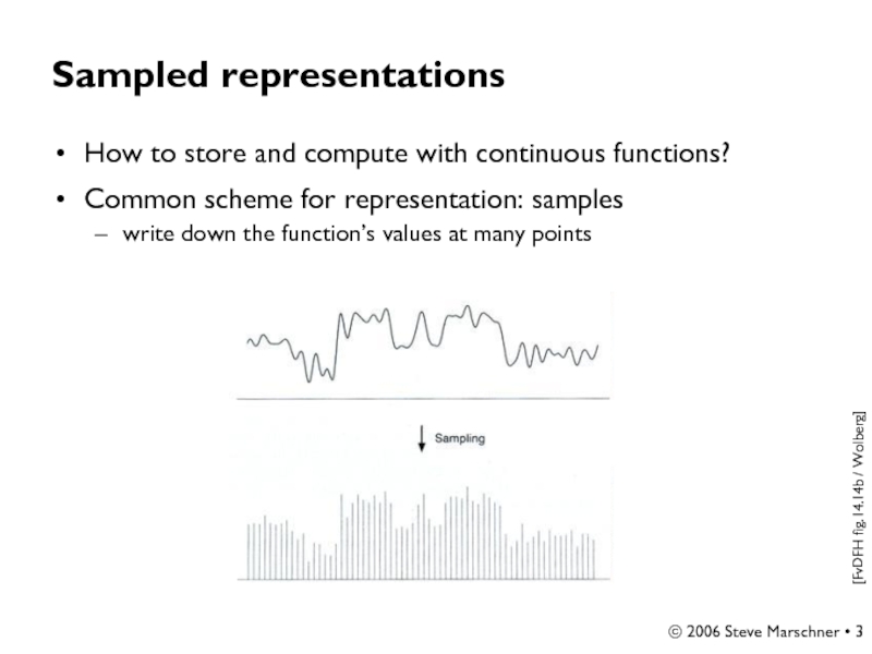
- 3. © 2006 Steve Marschner • Sampled
- 4. © 2006 Steve Marschner • Reconstruction
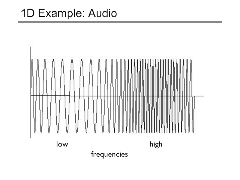
- 5. 1D Example: Audio low high frequencies
- 6. © 2006 Steve Marschner • Sampling
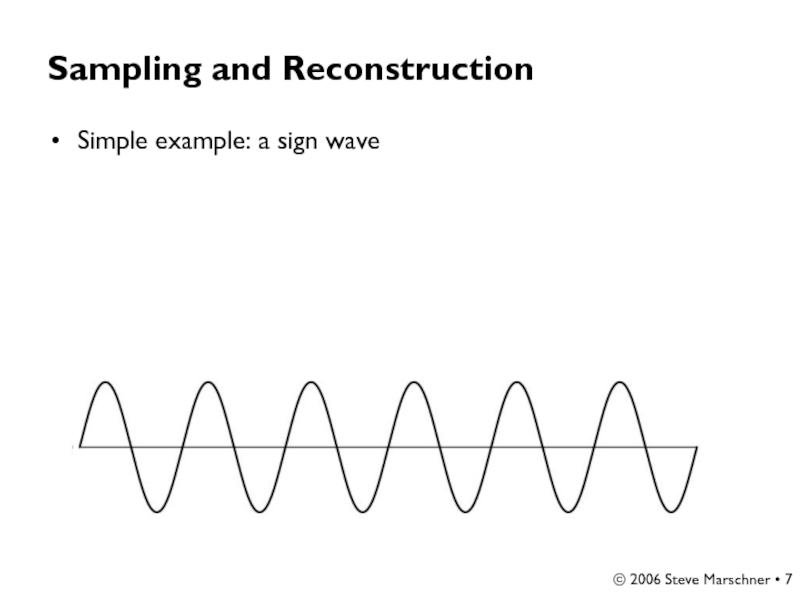
- 7. © 2006 Steve Marschner • Sampling and Reconstruction Simple example: a sign wave
- 8. © 2006 Steve Marschner • Undersampling
- 9. © 2006 Steve Marschner • Undersampling
- 10. © 2006 Steve Marschner • Undersampling
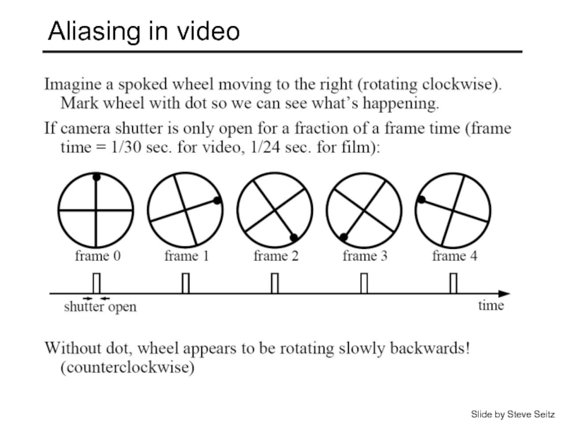
- 11. Aliasing in video Slide by Steve Seitz
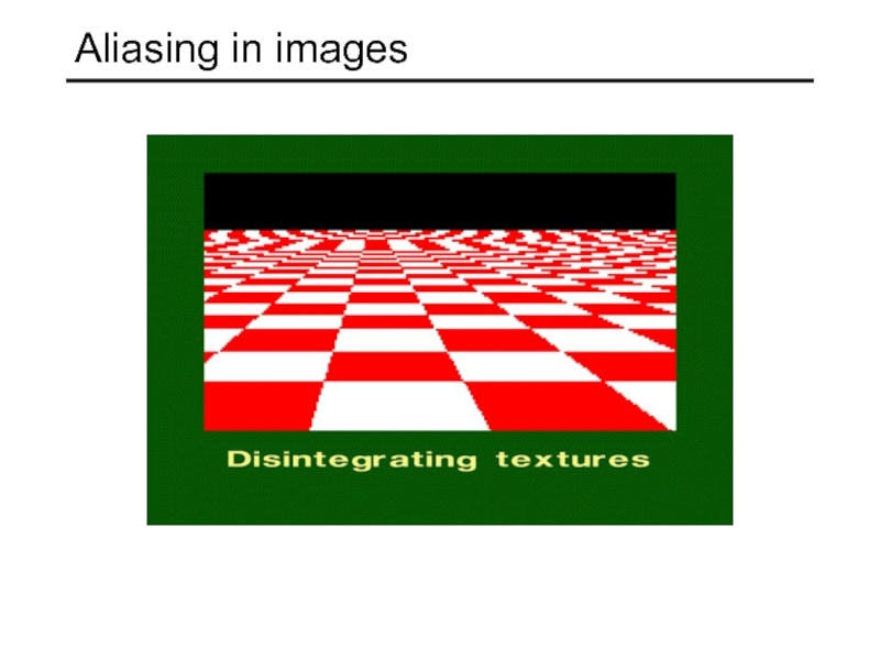
- 12. Aliasing in images
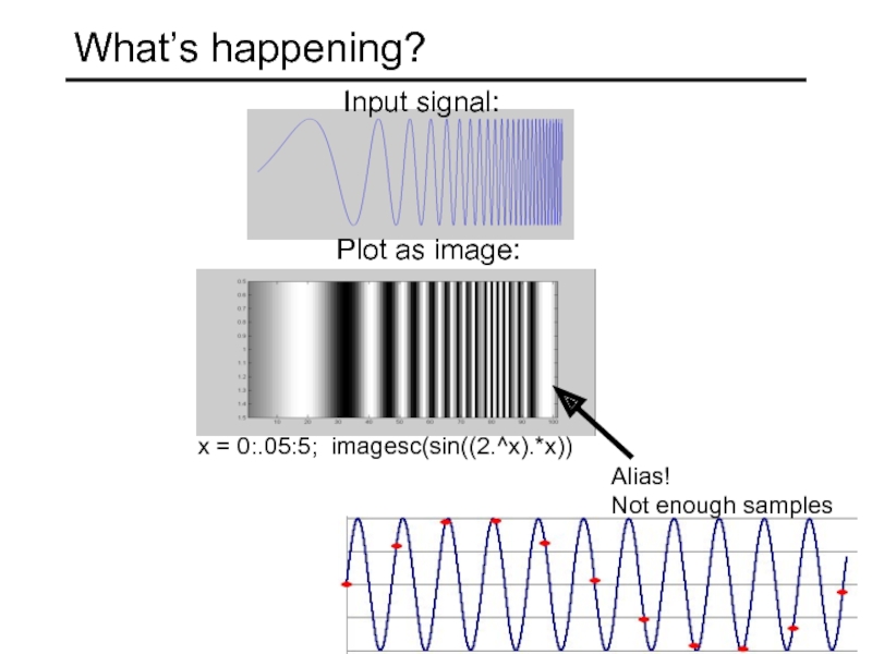
- 13. What’s happening? x = 0:.05:5; imagesc(sin((2.^x).*x)) Plot as image: Alias! Not enough samples
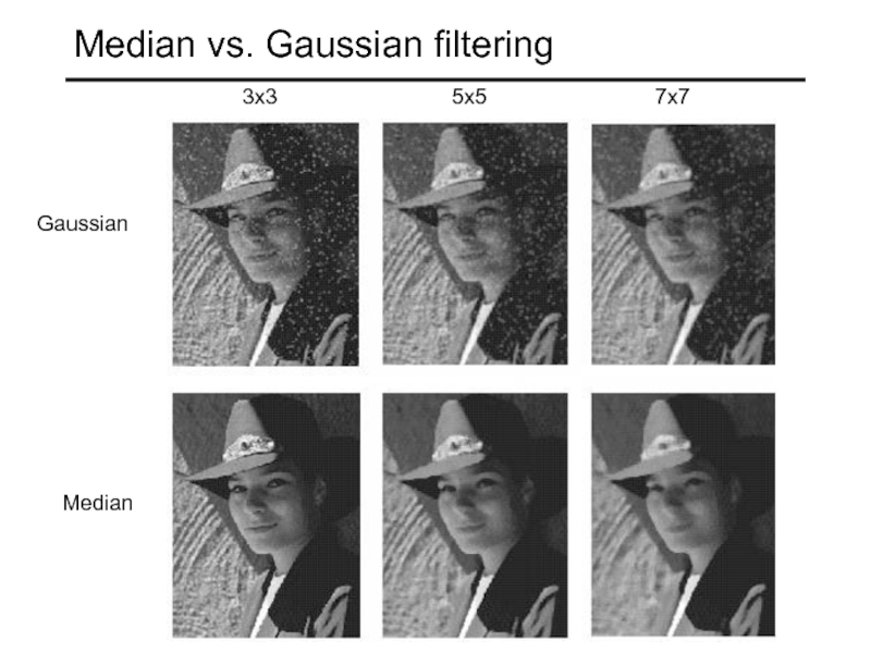
- 14. Antialiasing What can we do about aliasing?
- 15. © 2006 Steve Marschner • Preventing
- 16. © 2006 Steve Marschner • Linear
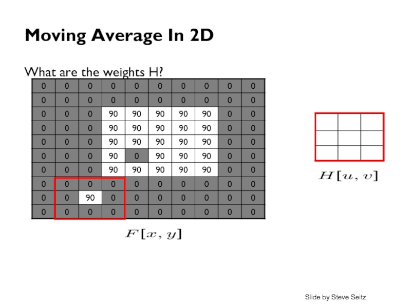
- 17. © 2006 Steve Marschner • Moving
- 18. © 2006 Steve Marschner • Weighted
- 19. © 2006 Steve Marschner • Weighted
- 20. © 2006 Steve Marschner • Moving
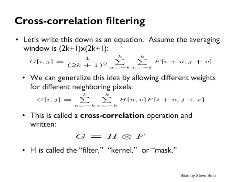
- 21. © 2006 Steve Marschner • Cross-correlation
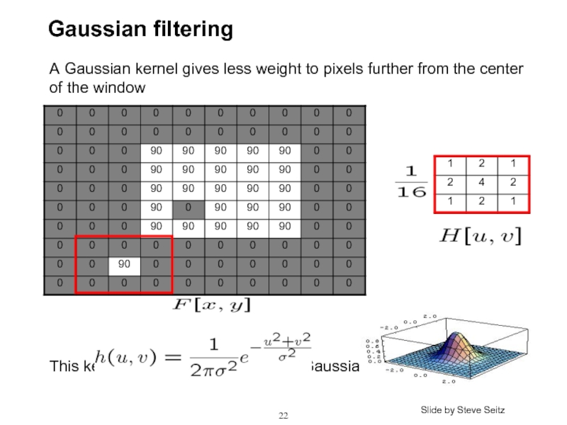
- 22. Gaussian filtering A Gaussian kernel gives less
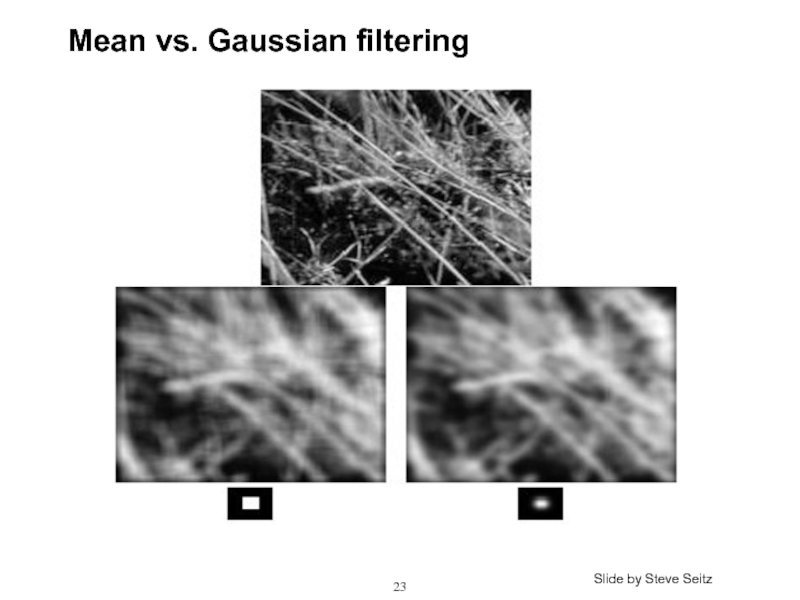
- 23. Mean vs. Gaussian filtering Slide by Steve Seitz
- 24. Convolution cross-correlation: A convolution
- 25. © 2006 Steve Marschner • Convolution
- 26. Tricks with convolutions =
- 27. Practice with linear filters Original ? Source: D. Lowe
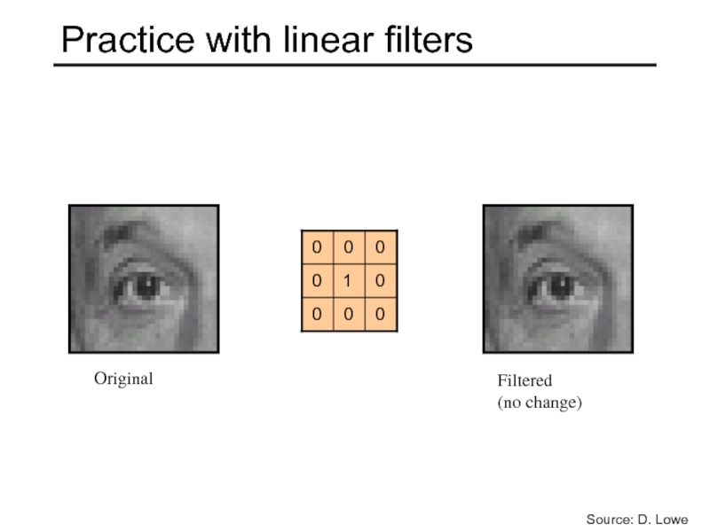
- 28. Practice with linear filters Original Filtered (no change) Source: D. Lowe
- 29. Practice with linear filters Original ? Source: D. Lowe
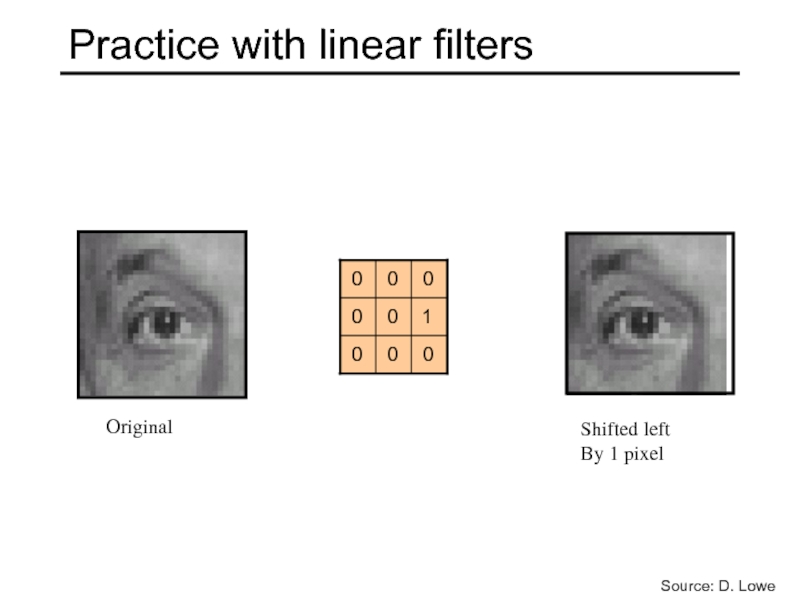
- 30. Practice with linear filters Original Shifted left By 1 pixel Source: D. Lowe
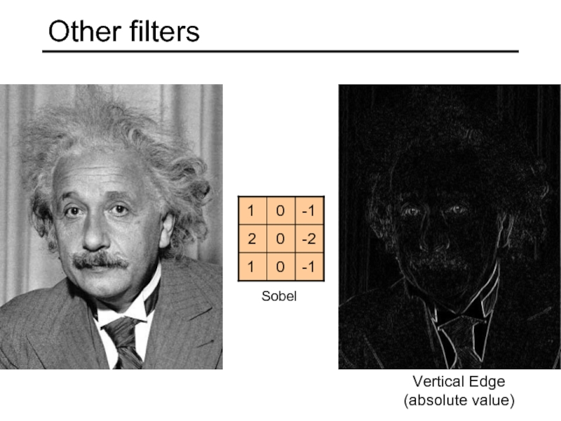
- 31. Other filters Vertical Edge (absolute value) Sobel
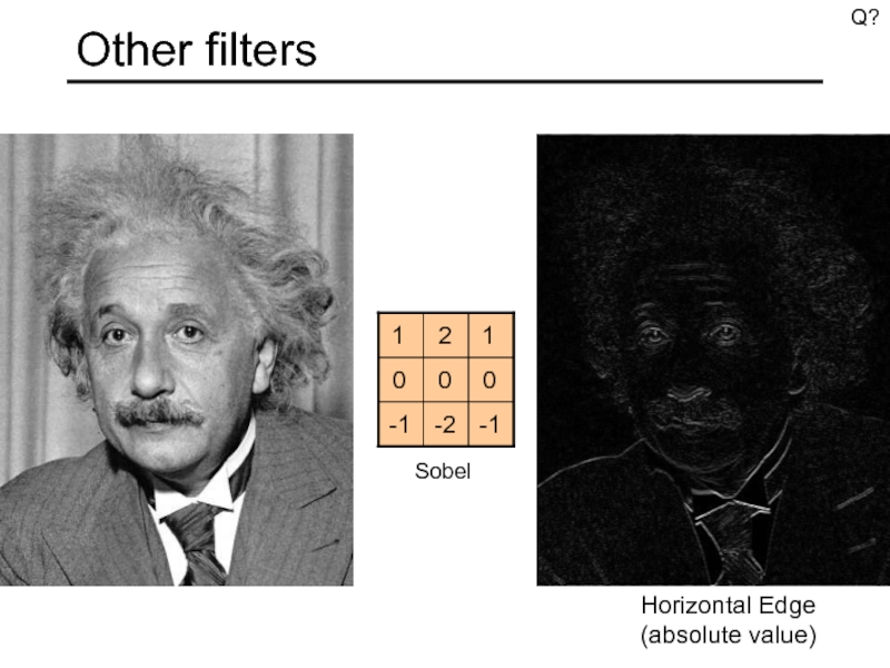
- 32. Other filters Horizontal Edge (absolute value) Sobel Q?
- 33. Weight contributions of neighboring pixels by nearness
- 34. Gaussian filters Remove “high-frequency” components from the
- 35. How big should the filter be? Values
- 36. Practical matters What is the size
- 37. Practical matters What about near the edge?
- 38. Practical matters methods (MATLAB):
- 39. Template matching Goal: find
- 40. Matching with filters Goal: find
- 41. Matching with filters Goal: find
- 42. Matching with filters Goal: find
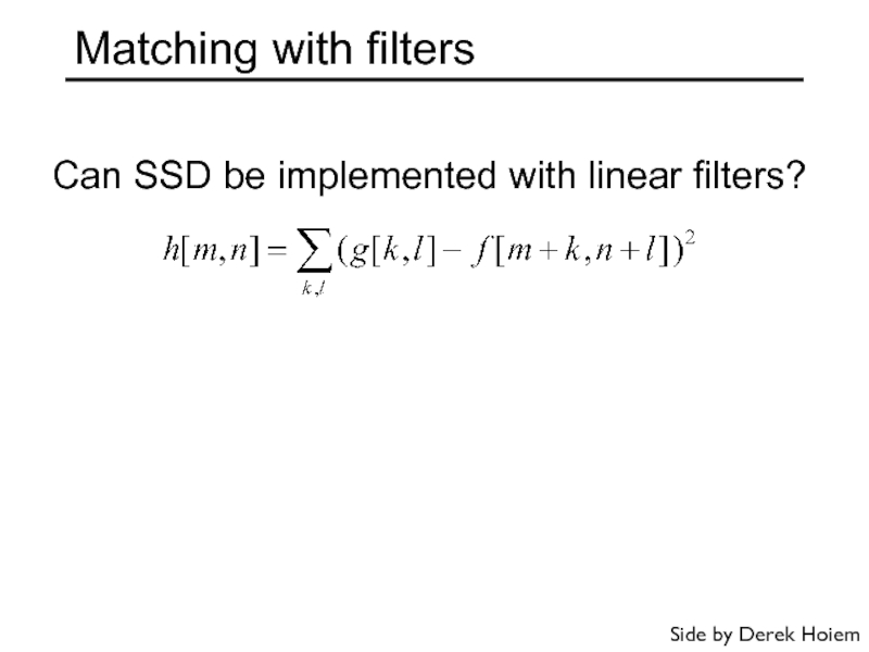
- 43. Matching with filters Can SSD be implemented with linear filters? Side by Derek Hoiem
- 44. Matching with filters Goal: find
- 45. Matching with filters Goal: find
- 46. Matching with filters Goal: find
- 47. Matching with filters Goal: find
- 48. Q: What is the best method to
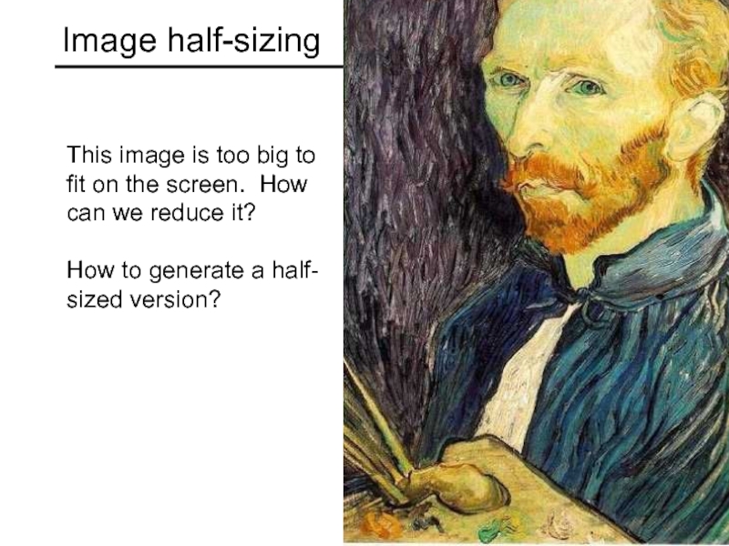
- 49. Image half-sizing This image is too big
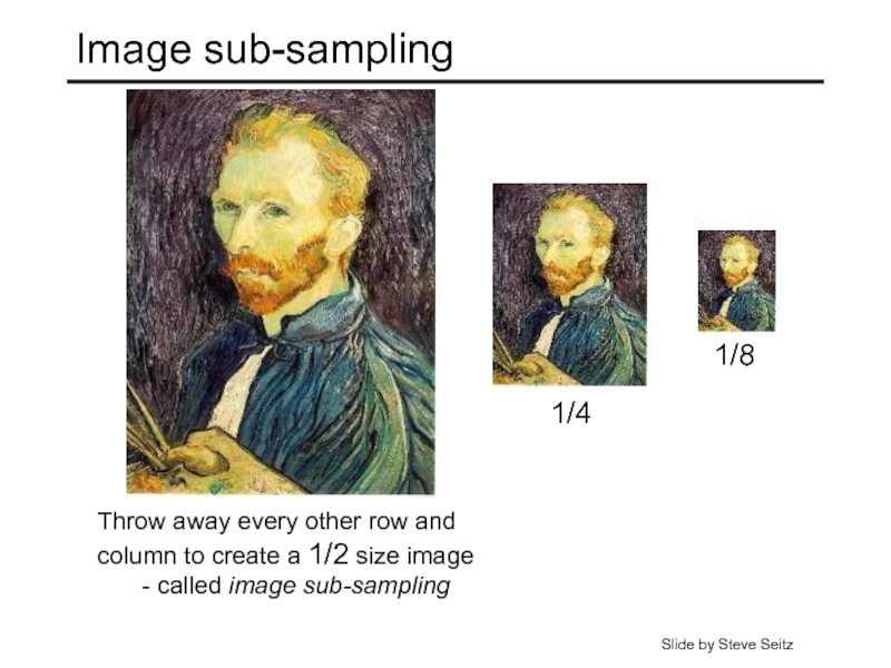
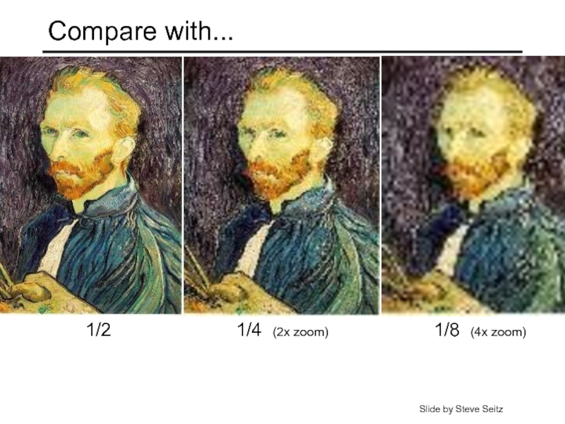
- 50. Image sub-sampling Throw away every other row
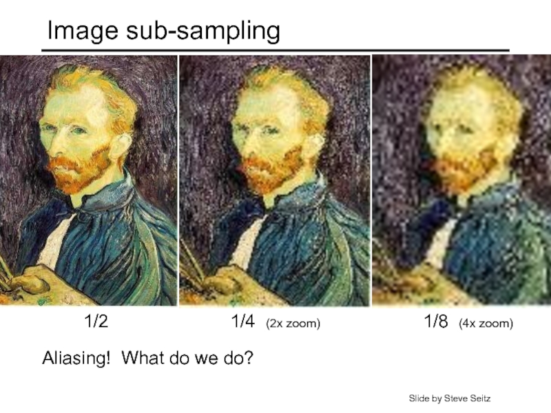
- 51. Image sub-sampling 1/4 (2x zoom) 1/8 (4x
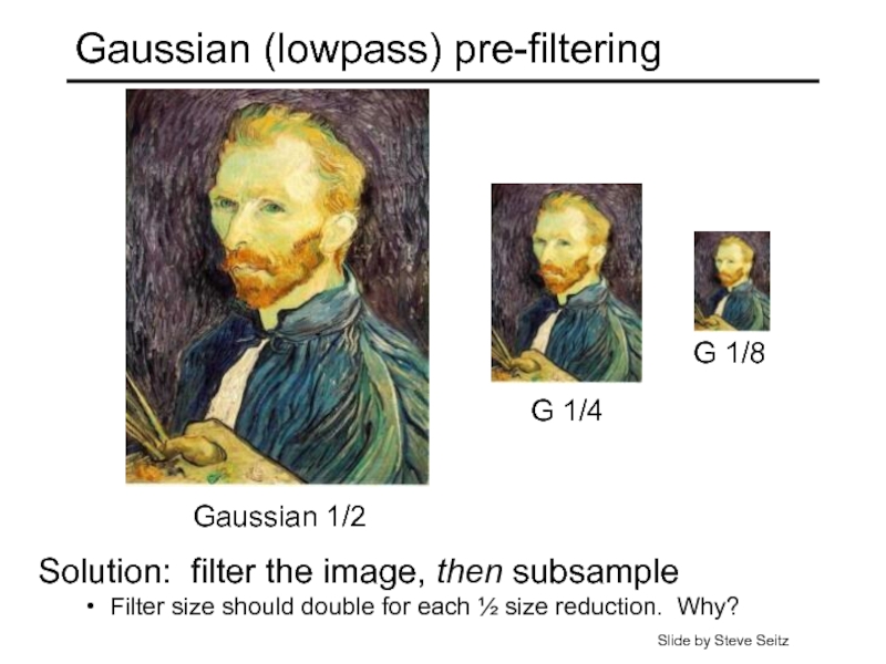
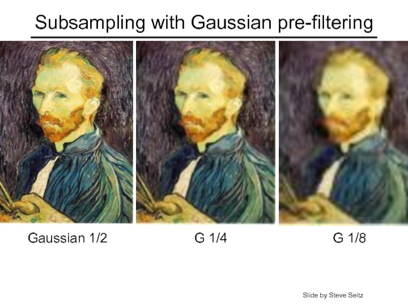
- 52. Gaussian (lowpass) pre-filtering G 1/4 G 1/8
- 53. Subsampling with Gaussian pre-filtering G 1/4 G 1/8 Gaussian 1/2 Slide by Steve Seitz
- 54. Compare with... 1/4 (2x zoom) 1/8 (4x zoom) 1/2 Slide by Steve Seitz
- 55. Gaussian (lowpass) pre-filtering G 1/4 G 1/8
- 56. Image Pyramids Known as a Gaussian Pyramid
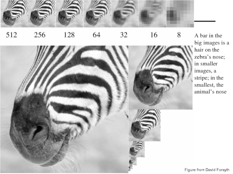
- 57. A bar in the big images is
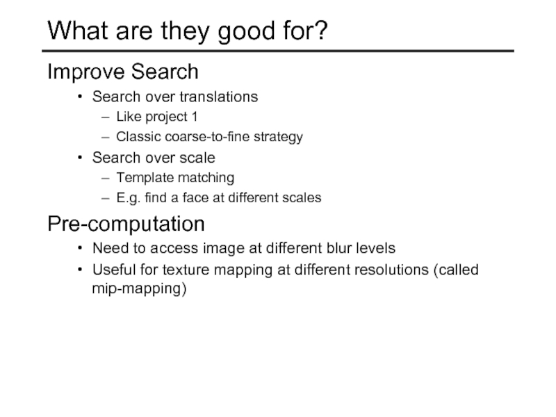
- 58. What are they good for? Improve Search
- 59. Gaussian pyramid construction
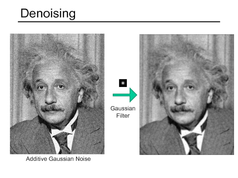
- 60. Denoising Additive Gaussian Noise Gaussian Filter
- 61. Smoothing with larger standard deviations suppresses noise,
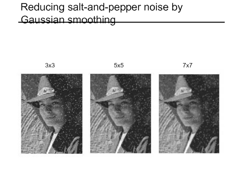
- 62. Reducing salt-and-pepper noise by Gaussian smoothing 3x3 5x5 7x7
- 63. Alternative idea: Median filtering A median filter
- 64. Median filter What advantage does median filtering
- 65. Median filter Salt-and-pepper noise Median filtered Source: M. Hebert MATLAB: medfilt2(image, [h w])
- 66. Median vs. Gaussian filtering 3x3 5x5 7x7 Gaussian Median
Слайд 115-463: Computational Photography
Alexei Efros, CMU, Fall 2012
Many slides from
Steve Marschner
Sampling
Слайд 3© 2006 Steve Marschner •
Sampled representations
How to store and compute
Common scheme for representation: samples
write down the function’s values at many points
[FvDFH fig.14.14b / Wolberg]
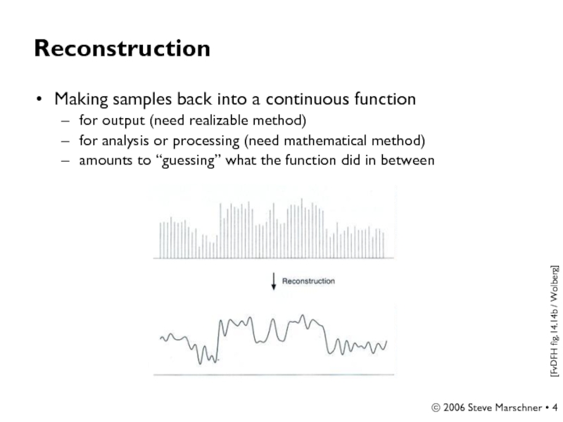
Слайд 4© 2006 Steve Marschner •
Reconstruction
Making samples back into a continuous
for output (need realizable method)
for analysis or processing (need mathematical method)
amounts to “guessing” what the function did in between
[FvDFH fig.14.14b / Wolberg]
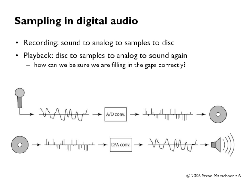
Слайд 6© 2006 Steve Marschner •
Sampling in digital audio
Recording: sound to
Playback: disc to samples to analog to sound again
how can we be sure we are filling in the gaps correctly?
Слайд 8© 2006 Steve Marschner •
Undersampling
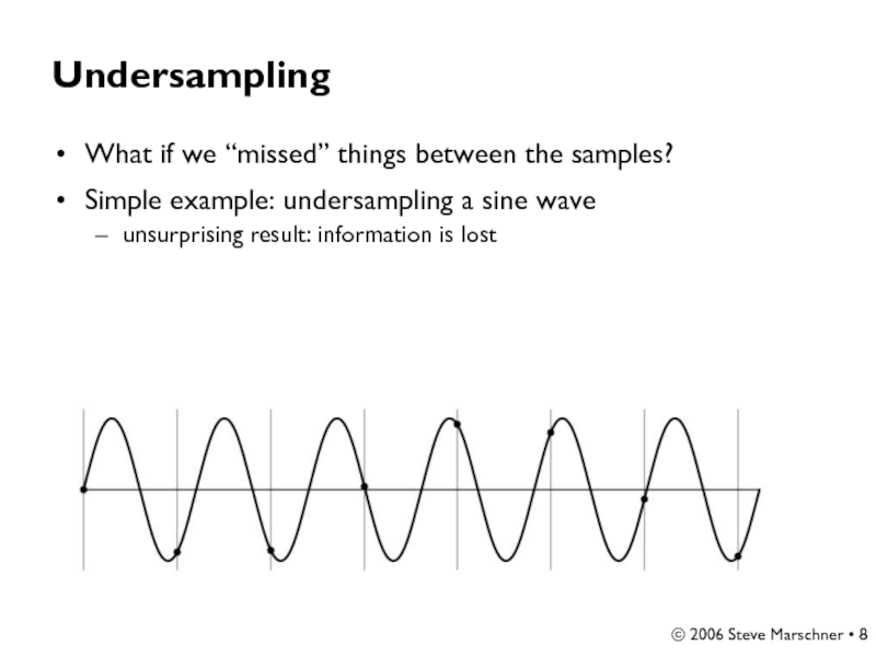
What if we “missed” things between
Simple example: undersampling a sine wave
unsurprising result: information is lost
Слайд 9© 2006 Steve Marschner •
Undersampling
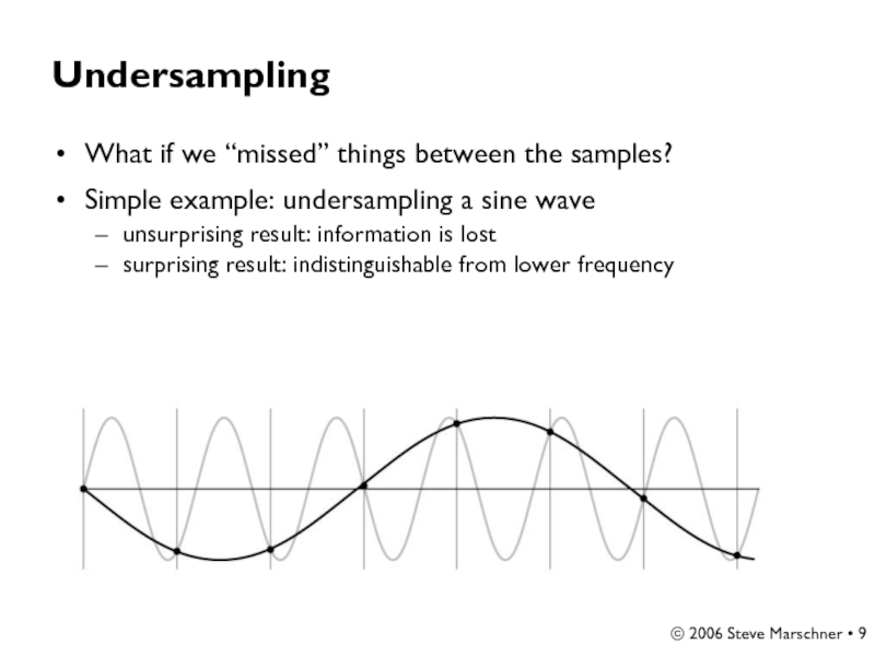
What if we “missed” things between
Simple example: undersampling a sine wave
unsurprising result: information is lost
surprising result: indistinguishable from lower frequency
Слайд 10© 2006 Steve Marschner •
Undersampling
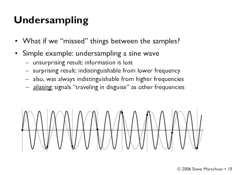
What if we “missed” things between
Simple example: undersampling a sine wave
unsurprising result: information is lost
surprising result: indistinguishable from lower frequency
also, was always indistinguishable from higher frequencies
aliasing: signals “traveling in disguise” as other frequencies
Слайд 14Antialiasing
What can we do about aliasing?
Sample more often
Join the Mega-Pixel craze
But this can’t go on forever
Make the signal less “wiggly”
Get rid of some high frequencies
Will loose information
But it’s better than aliasing
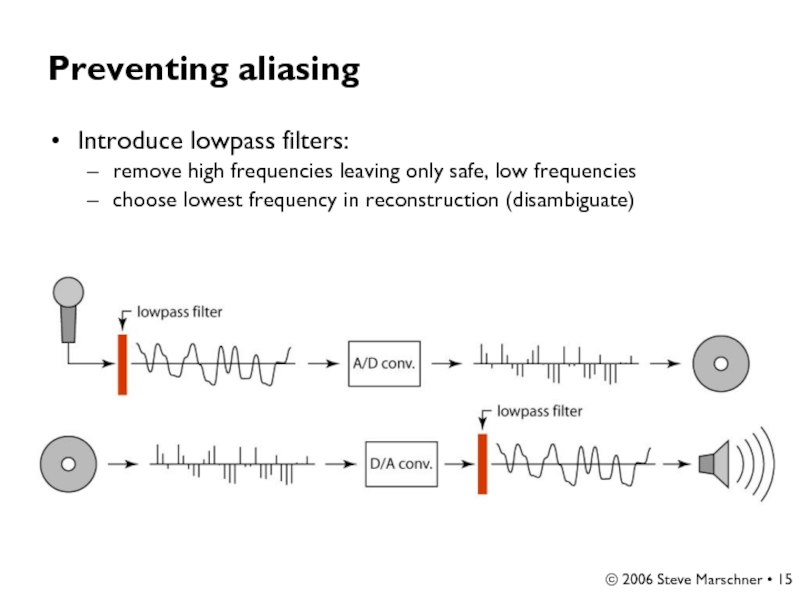
Слайд 15© 2006 Steve Marschner •
Preventing aliasing
Introduce lowpass filters:
remove high frequencies
choose lowest frequency in reconstruction (disambiguate)
Слайд 16© 2006 Steve Marschner •
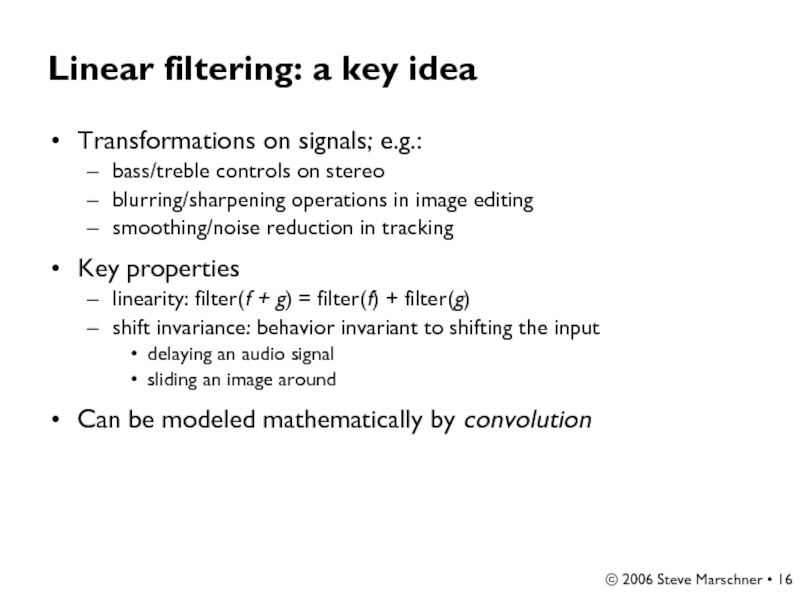
Linear filtering: a key idea
Transformations on
bass/treble controls on stereo
blurring/sharpening operations in image editing
smoothing/noise reduction in tracking
Key properties
linearity: filter(f + g) = filter(f) + filter(g)
shift invariance: behavior invariant to shifting the input
delaying an audio signal
sliding an image around
Can be modeled mathematically by convolution
Слайд 17© 2006 Steve Marschner •
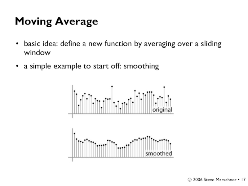
Moving Average
basic idea: define a new
a simple example to start off: smoothing
Слайд 18© 2006 Steve Marschner •
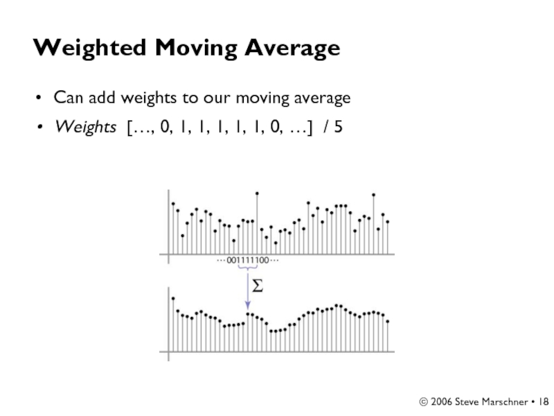
Weighted Moving Average
Can add weights to
Weights […, 0, 1, 1, 1, 1, 1, 0, …] / 5
Слайд 19© 2006 Steve Marschner •
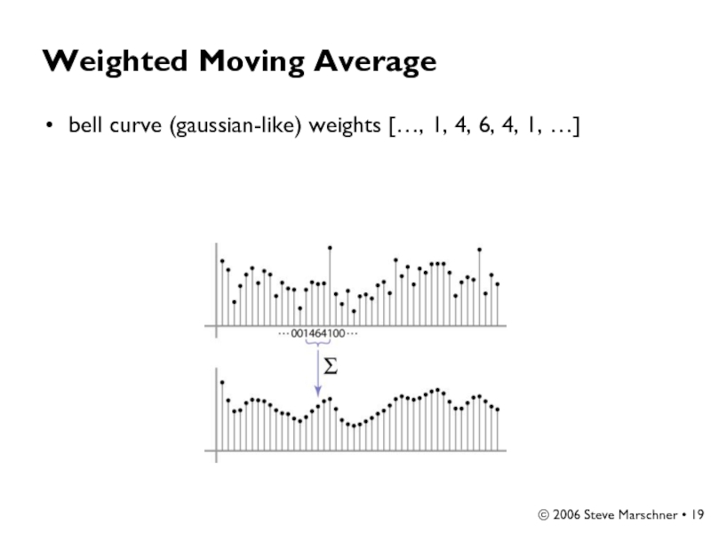
Weighted Moving Average
bell curve (gaussian-like) weights
Слайд 21© 2006 Steve Marschner •
Cross-correlation filtering
Let’s write this down as
We can generalize this idea by allowing different weights for different neighboring pixels:
This is called a cross-correlation operation and
written:
H is called the “filter,” “kernel,” or “mask.”
Slide by Steve Seitz
Слайд 22Gaussian filtering
A Gaussian kernel gives less weight to pixels further from
This kernel is an approximation of a Gaussian function:
Slide by Steve Seitz
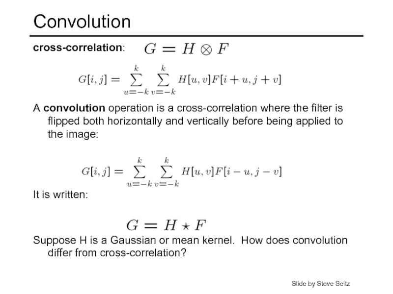
Слайд 24Convolution
cross-correlation:
A convolution operation is a cross-correlation where the filter is flipped
It is written:
Suppose H is a Gaussian or mean kernel. How does convolution differ from cross-correlation?
Slide by Steve Seitz
Слайд 25© 2006 Steve Marschner •
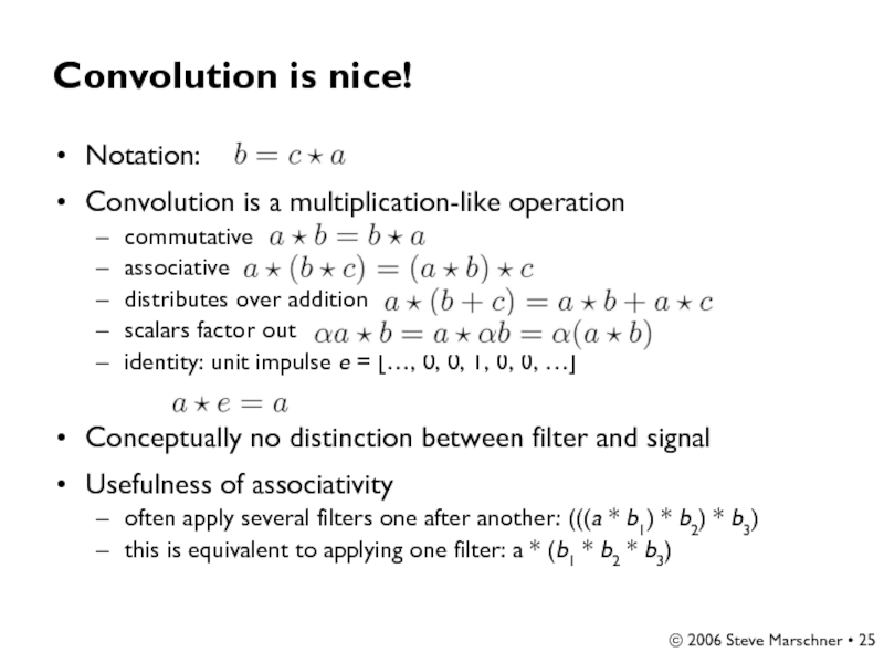
Convolution is nice!
Notation:
Convolution is a multiplication-like
commutative
associative
distributes over addition
scalars factor out
identity: unit impulse e = […, 0, 0, 1, 0, 0, …]
Conceptually no distinction between filter and signal
Usefulness of associativity
often apply several filters one after another: (((a * b1) * b2) * b3)
this is equivalent to applying one filter: a * (b1 * b2 * b3)
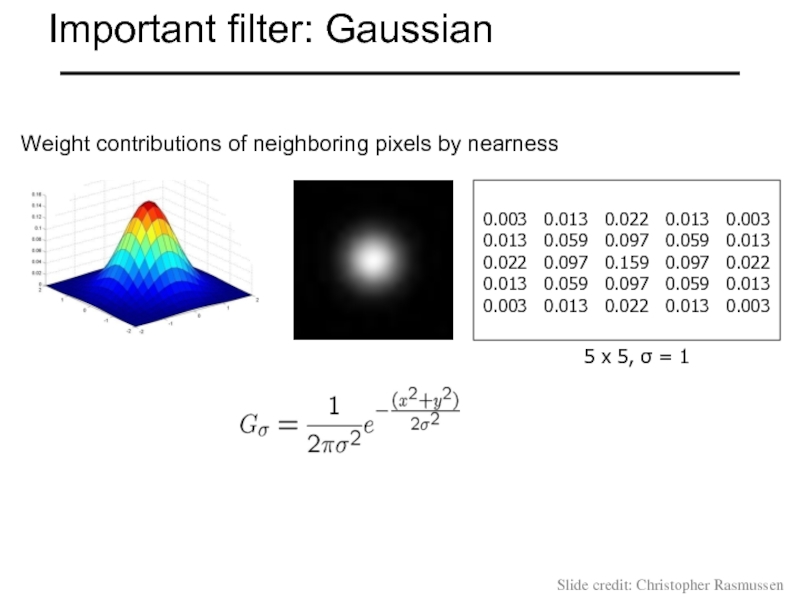
Слайд 33Weight contributions of neighboring pixels by nearness
0.003 0.013 0.022
0.013 0.059 0.097 0.059 0.013
0.022 0.097 0.159 0.097 0.022
0.013 0.059 0.097 0.059 0.013
0.003 0.013 0.022 0.013 0.003
5 x 5, σ = 1
Slide credit: Christopher Rasmussen
Important filter: Gaussian
Слайд 34Gaussian filters
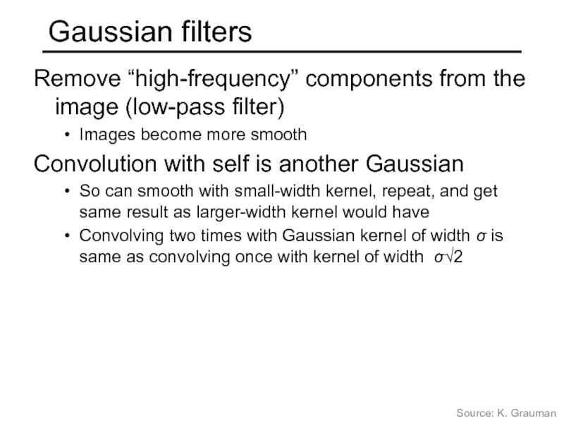
Remove “high-frequency” components from the image (low-pass filter)
Images become more
Convolution with self is another Gaussian
So can smooth with small-width kernel, repeat, and get same result as larger-width kernel would have
Convolving two times with Gaussian kernel of width σ is same as convolving once with kernel of width σ√2
Source: K. Grauman
Слайд 35How big should the filter be?
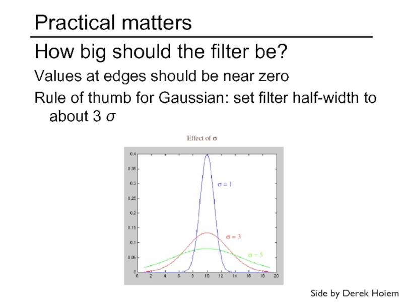
Values at edges should be near
Rule of thumb for Gaussian: set filter half-width to about 3 σ
Practical matters
Side by Derek Hoiem
Слайд 36
Practical matters
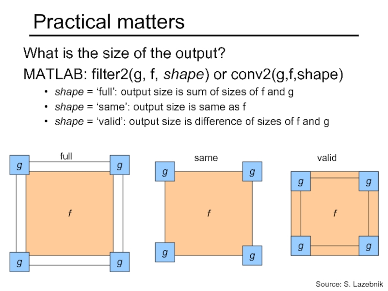
What is the size of the output?
MATLAB: filter2(g, f, shape)
shape = ‘full’: output size is sum of sizes of f and g
shape = ‘same’: output size is same as f
shape = ‘valid’: output size is difference of sizes of f and g
f
g
g
g
g
f
g
g
g
g
f
g
g
g
g
full
same
valid
Source: S. Lazebnik
Слайд 37Practical matters
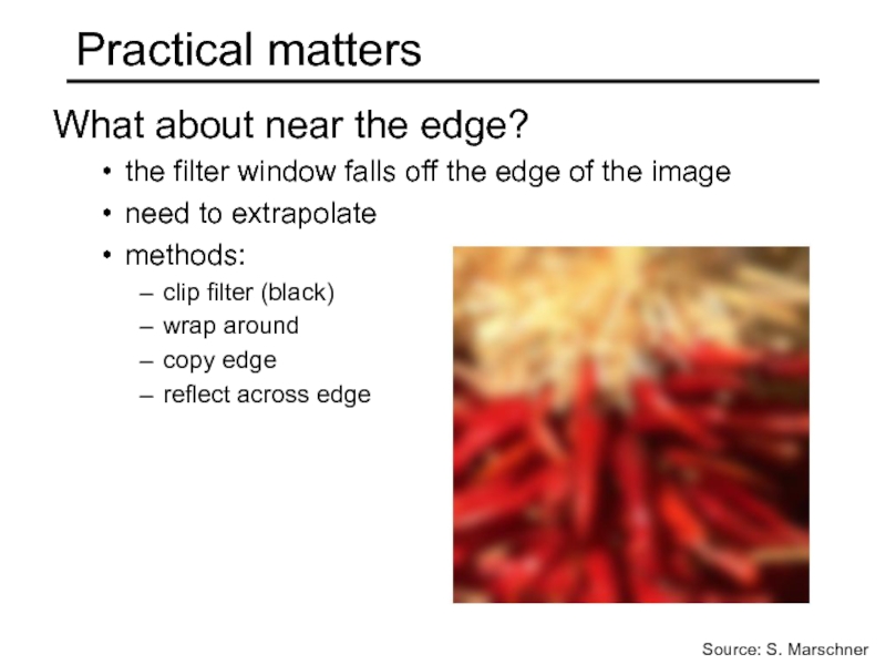
What about near the edge?
the filter window falls off the
need to extrapolate
methods:
clip filter (black)
wrap around
copy edge
reflect across edge
Source: S. Marschner
Слайд 38Practical matters
methods (MATLAB):
clip filter (black): imfilter(f, g, 0)
wrap around: imfilter(f, g, ‘circular’)
copy
reflect across edge: imfilter(f, g, ‘symmetric’)
Source: S. Marschner
Q?
Слайд 39Template matching
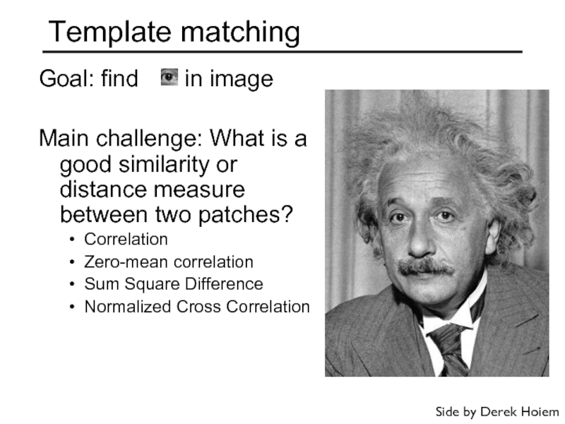
Goal: find in image
Main challenge: What is
Correlation
Zero-mean correlation
Sum Square Difference
Normalized Cross Correlation
Side by Derek Hoiem
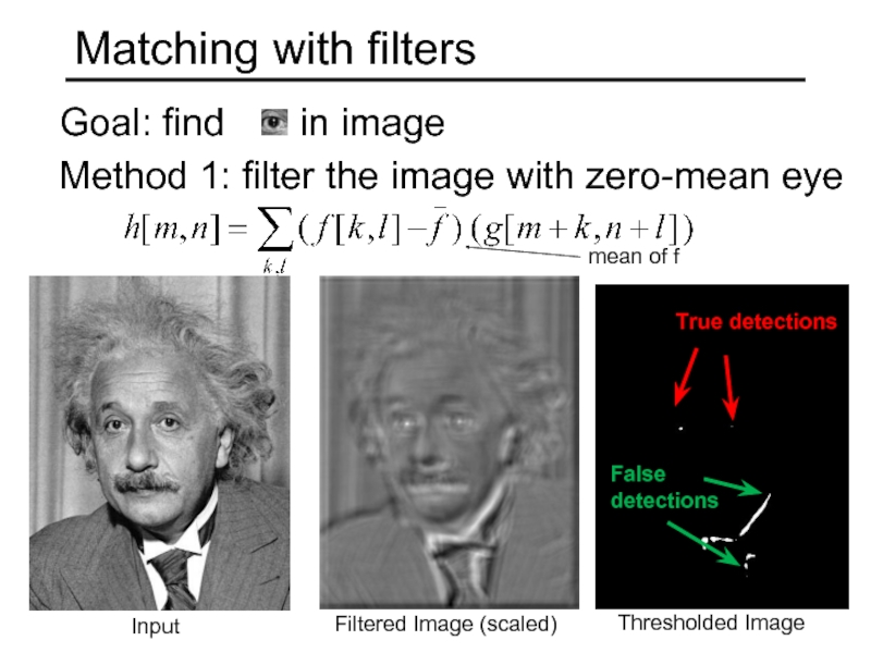
Слайд 40Matching with filters
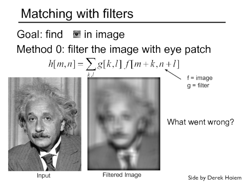
Goal: find in image
Method 0: filter
Input
Filtered Image
What went wrong?
f = image
g = filter
Side by Derek Hoiem
Слайд 41Matching with filters
Goal: find in image
Method 1: filter
Input
Filtered Image (scaled)
Thresholded Image
True detections
False detections
mean of f
Слайд 42Matching with filters
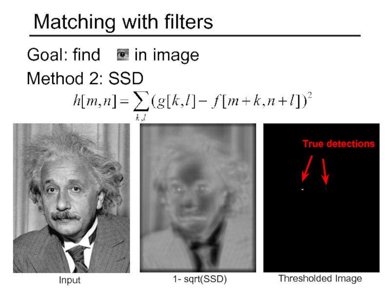
Goal: find in image
Method 2: SSD
Input
1-
Thresholded Image
True detections
Слайд 44Matching with filters
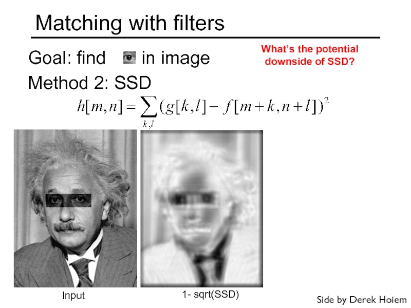
Goal: find in image
Method 2: SSD
Input
1-
What’s the potential downside of SSD?
Side by Derek Hoiem
Слайд 45Matching with filters
Goal: find in image
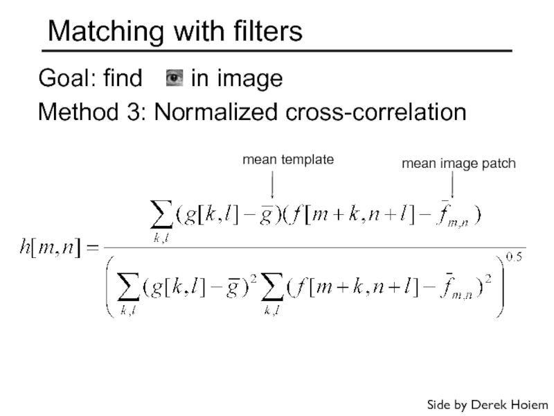
Method 3: Normalized
mean image patch
mean template
Side by Derek Hoiem
Слайд 46Matching with filters
Goal: find in image
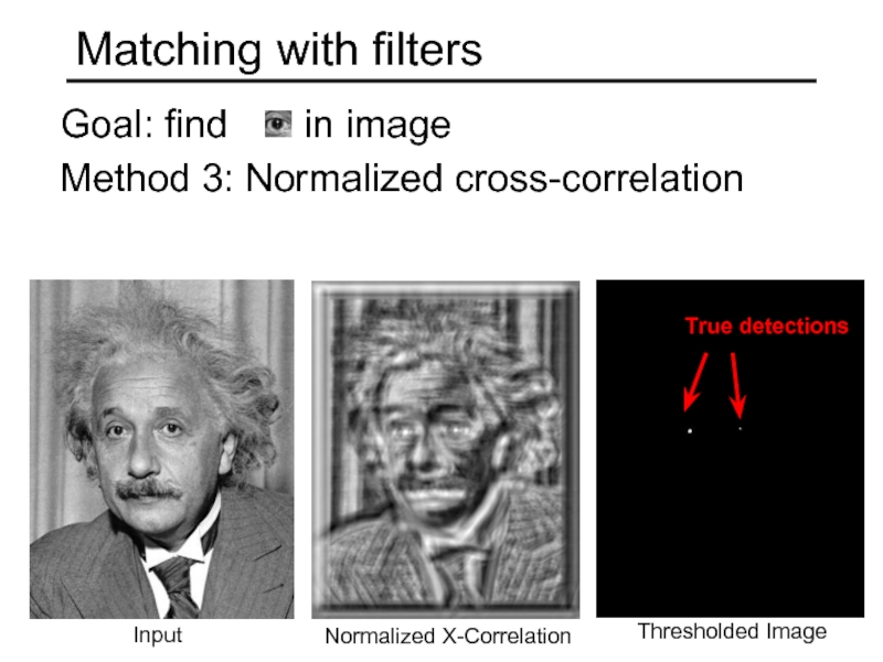
Method 3: Normalized
Input
Normalized X-Correlation
Thresholded Image
True detections
Слайд 47Matching with filters
Goal: find in image
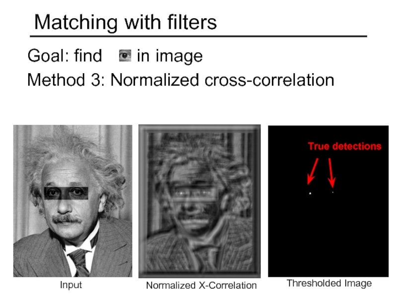
Method 3: Normalized
Input
Normalized X-Correlation
Thresholded Image
True detections
Слайд 48Q: What is the best method to use?
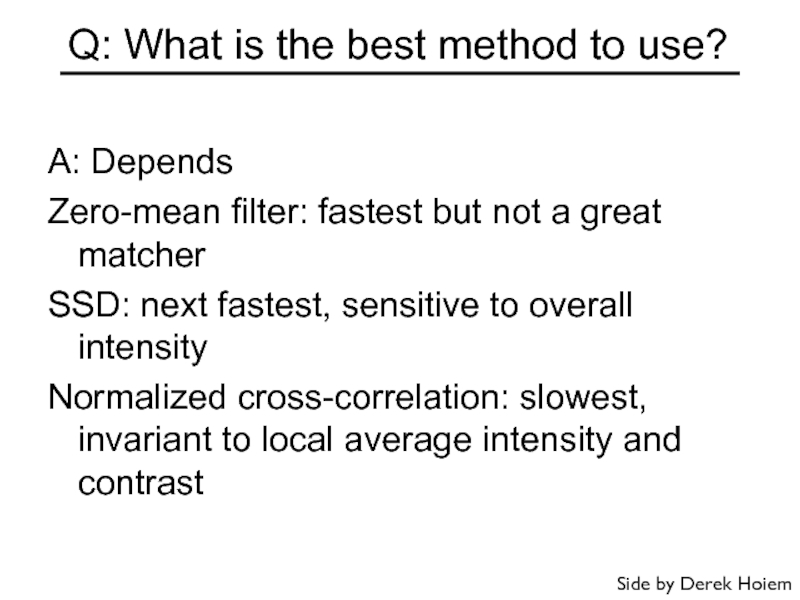
A: Depends
Zero-mean filter: fastest
SSD: next fastest, sensitive to overall intensity
Normalized cross-correlation: slowest, invariant to local average intensity and contrast
Side by Derek Hoiem
Слайд 49Image half-sizing
This image is too big to
fit on the screen. How
can
How to generate a half-
sized version?
Слайд 50Image sub-sampling
Throw away every other row and column to create a
- called image sub-sampling
1/4
1/8
Slide by Steve Seitz
Слайд 52Gaussian (lowpass) pre-filtering
G 1/4
G 1/8
Gaussian 1/2
Solution: filter the image, then subsample
Filter
Slide by Steve Seitz
Слайд 55Gaussian (lowpass) pre-filtering
G 1/4
G 1/8
Gaussian 1/2
Solution: filter the image, then subsample
Filter
How can we speed this up?
Slide by Steve Seitz
Слайд 56Image Pyramids
Known as a Gaussian Pyramid [Burt and Adelson, 1983]
In computer
A precursor to wavelet transform
Slide by Steve Seitz
Слайд 57A bar in the big images is a hair on the
Figure from David Forsyth
Слайд 58What are they good for?
Improve Search
Search over translations
Like project 1
Classic coarse-to-fine
Search over scale
Template matching
E.g. find a face at different scales
Pre-computation
Need to access image at different blur levels
Useful for texture mapping at different resolutions (called mip-mapping)
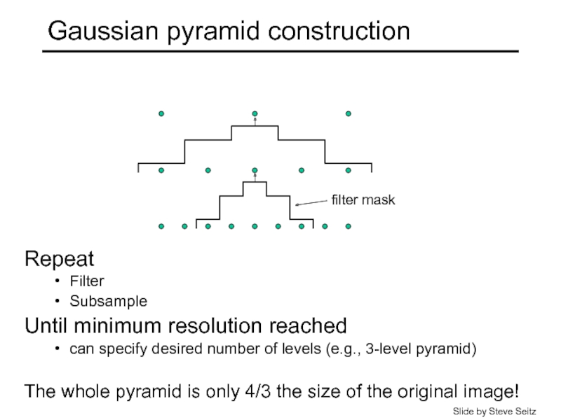
Слайд 59Gaussian pyramid construction
filter mask
Repeat
Filter
Subsample
Until minimum resolution reached
can specify desired number
The whole pyramid is only 4/3 the size of the original image!
Slide by Steve Seitz
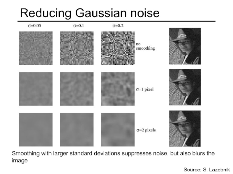
Слайд 61Smoothing with larger standard deviations suppresses noise, but also blurs the
Reducing Gaussian noise
Source: S. Lazebnik
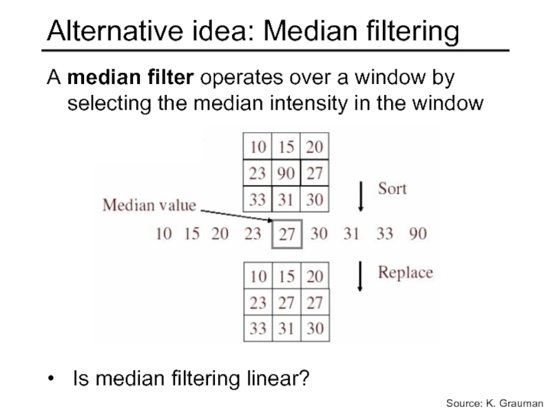
Слайд 63Alternative idea: Median filtering
A median filter operates over a window by
Is median filtering linear?
Source: K. Grauman
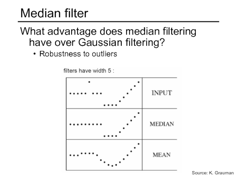
Слайд 64Median filter
What advantage does median filtering have over Gaussian filtering?
Robustness to
Source: K. Grauman



![Image PyramidsKnown as a Gaussian Pyramid [Burt and Adelson, 1983]In computer graphics, a mip map](/img/tmb/1/69794/8218a903e36a22ca807548111c2023f0-800x.jpg)
![Median filterSalt-and-pepper noiseMedian filteredSource: M. HebertMATLAB: medfilt2(image, [h w])](/img/tmb/1/69794/55e2cacd0e198a1bd5178b34f8e069a7-800x.jpg)
