Слайд 1Kazan National Research Technical University named after A.N. Tupolev
German-Russian Institute of
Advanced Technologies (GRIAT)
NEURAL NETWORKS
by Dr. Igor Anikin
Слайд 2Table of contents
The basic concepts of neural networks
Artificial neural networks.
The
structure of an artificial neuron.
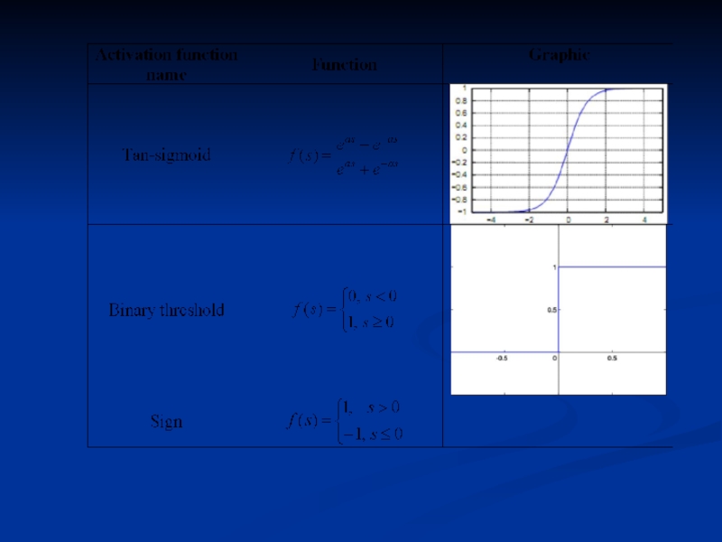
Activation functions.
Basic paradigms of neural networks.
Fundamentals of learning and training samples.
Using neural networks in practice
Single layer neural networks
Rosenblatt's single layer perceptron.
Learning single layer neural networks.
Associative memory and its realization on single layer neural networks.
Using single layer neural networks for pattern recognition and time series forecasing.
Multilayer perceptrons
The structure of multilayer perceptrons
Back propagation of error.
Using multilayer perceptrons for pattern recognition and time series forecasing.
Слайд 3Self-organizing maps
The principle of unsupervised learning.
Kohonen self-organizing maps.
Learning Kohonen
networks.
Practical using of Kohonen networks
Recurent neural networks
Neural networks with feedback.
Hopfield neural network.
Hamming neural network.
Training Hopfield and Hamming neural networks.
Practical using of Hopfield and Hamming neural networks.
Training and Testing
Training error and testing error.
Слайд 4References
David Kriesel. A brief Introduction to Neural networks // http://www.dkriesel.com/en/science/neural_networks
Raul
Rojas. Neural Networks. A Systematic Introduction // http://www.inf.fu-berlin.de/inst/ag-ki/rojas_home/documents/1996/NeuralNetworks/neuron.pdf.
L.P.J. Veelenturf. Analysis and Application of Artificial Neural Networks // http://www.ru.lv/~peter/zinatne/ebooks/Analysis%20and%20Applications%20of%20Artificial%20Neural%20Networks.pdf
Artificial Neural Networks – Methodological Advances and Biomedical Applications // InTech.ORG
Слайд 5The basic concepts of neural networks
Слайд 6Questions for motivation discussion
What tasks are machines good at doing that
humans are not?
What tasks are humans good at doing that machines are not?
What tasks are both good at?
What does it mean to learn?
How is learning related to intelligence?
What does it mean to be intelligent?
Do you believe a machine will ever been intelligent?
If a computer were intelligent, how would you know?
Слайд 7Types of learning
Knowledge acquisition from expert.
Knowledge acquisition from data:
Supervised learning –
the system is supplied with a set of training examples consisting of inputs and corresponding outputs, and is required to discover the relation or mapping between them.
Unsupervised learning – the system is supplied with a set of training examples consisting only of inputs. It is required to discover what appropriate outputs should be.
Слайд 8Artificial Neural Network
An extremely simplified model of the human’s brain
Transforms inputs
into the best outputs (some neural networks are the universal function approximators).
Слайд 9Artificial Neural Networks
Development of Neural Networks date back to the early
1940s.
It experienced an upsurge in popularity in the late 1980s due to discovery of new techniques of NN training.
Some NNs are models of biological neural networks and some are not, but historically, much of the inspiration for the field of NNs came from the desire to produce artificial systems capable of sophisticated, perhaps intelligent, computations similar to those that the human brain routinely performs, and thereby possibly to enhance our understanding of the human brain.
Most NNs have some sort of training rule. In other words, NNs learn from the examples (as children learn to recognize dogs from examples of dogs) and exhibit some capability for generalization beyond the training data.
Слайд 10ANN vs Computers
Computers have to be explicitly programmed
Analyze the problem to
be solved.
Write the code in a programming language.
Neural networks learn from the examples
No requirement of an explicit description of the problem.
No need for a programmer.
The neural computer adapts itself during a training period, based on examples of similar problems even without a desired solution to each problem. After sufficient training the neural computer is able to relate the problem data to the solutions, inputs to outputs, and it is then able to offer a viable solution to a brand new problem.
Слайд 11ANN vs Computers
Digital Computers
Deductive Reasoning. We apply known rules to input
data to produce output.
Computation is centralized, synchronous, and serial.
Memory is literally stored, and location addressable.
Not fault tolerant. One transistor goes and it no longer works.
Exact.
Static connectivity.
Applicable if well-defined rules accessible with precise input data.
Neural Networks
Inductive Reasoning. We use given input and output data (training examples) to make a reasoning.
Computation is collective, asynchronous, and parallel.
Memory is distributed, internalized, short term and content addressable.
Fault tolerant, redundancy, and sharing of responsibilities.
Inexact.
Dynamic connectivity.
Applicable if rules are unknown or complicated, or if data are noisy or partial.
Слайд 13Biological neuron
Many “neurons” co-operate to perform the desired function
Basic elements:
Axon
Dendrite
Synapse
Слайд 14Artificial Neuron Structure
The output of a neuron is a function of
the weighted sum of the inputs plus a bias
Слайд 17Examples of ANN topologies
Single layer ANN
Multilayer ANN
ANN with one recurrent layer
Слайд 18Fundamentals of learning and training samples
The weights in a neural
network are the most important factor in determining its function.
A training set is a set of training patterns, which we use to train our neural net.
Training is the act of presenting the network with some sample data and modifying the weights to better approximate the desired function
Слайд 19Fundamentals of learning and training samples
There are two main types
of training
Supervised Training
Supplies the neural network with inputs and the correct outputs (results).
We can estimate a error vector for certain input.
Response of the network to the inputs is measured. The weights are modified to reduce the difference between the actual and desired outputs
Unsupervised Training
The training set only consists of input patterns.
The neural network adjusts its own weights so that similar inputs cause similar outputs. The network identifies the patterns and differences in the inputs without any external assistance
Слайд 20Fundamentals of learning and training samples
A training pattern is an
input vector p with the components x1, x2, . . . , xn whose desired output is known.
By entering the training pattern into the network we receive an output that can be compared with the desired output.
The set of training patterns is called P. It contains a finite number of ordered pairs (p, t) of training patterns with corresponding desired output t.
Слайд 21Fundamentals of learning and training samples
Teaching input. Let j be an
output neuron. The teaching input tj is the desired and correct value j should output after the input of a certain training pattern.
Analogously to the vector p the teaching inputs t1, t2, . . . , tn of the neurons can also be combined into a vector t. This vector always refers to a specific training pattern p and contained in the set P of the training patterns.
Слайд 22Fundamentals of learning and training samples
Error vector. For several output neurons
Ω1,Ω2, . . . ,ΩO the difference between output vector and teaching input under a training input p is referred to as error vector.
Слайд 23Fundamentals of learning
Let P be the set of training patters. In
learning procedure we realize finite number of iterations or epochs.
Epoch – single presentation of the entire data to the neural network. Typically many epochs are required to train the neural network
Iteration - the process of providing the network with an single input and updating the network's weights
Слайд 24General learning procedure
Let P be the set of n training
patters pn
For i=1 to n
begin
We calculate NN output vector yi for the training pattern pi.
We compare yi with desired output ti. Then we calculate the error of output and make modification of weights.
end
If total error for the training set P more than some threshold then go to the step 2
Слайд 25Using training samples
We have to divide the set of training samples
into two subsets:
one training set really used to train;
one verification set to test our progress of learning.
The usual division relations are, 70% for training data and 30% for verification data (randomly chosen).
We can finish the training process when the network provides the good results on the training data as well as on the verification data.
Слайд 26Learning curve
The learning curve indicates the progress of the error, which
can be determined in various ways. This curve can indicate whether the network is progressing or not.
Слайд 27Error measurement
Let Ω be the output neuron and O be the
set of output neurons.
The specific error Errp is based on a single training sample.
The total error Err is based on all training samples.
Слайд 28When do we stop learning?
Generally, the training process is stopped when
the user in front of the learning computer "thinks" the error is small enough.
Слайд 29Using neural networks in practice (discussion)
Classification
in marketing: consumer spending pattern
classification
In defence: radar and sonar image classification
In medicine: ultrasound and electrocardiogram image classification, EEGs, medical diagnosis
Recognition and identification
In general computing and telecommunications: speech, vision and handwriting recognition
In finance: signature verification and bank note verification
Assessment
In engineering: product inspection monitoring and control
In defence: target tracking
In security: motion detection, surveillance image analysis and fingerprint matching
Forecasting and prediction
In finance: foreign exchange rate and stock market forecasting
In agriculture: crop yield forecasting
In marketing: sales forecasting
In meteorology: weather prediction
Слайд 31Single layer network with binary threshold activation function
Matrix form
Слайд 32Single layer network with binary threshold activation function
Слайд 33Practice with single layer
neural network
Performing a calculations in single
layer neural networks with using direct and matrix form. Using various activation functions.
Using single layer neural networks with binary threshold activation function as linear classifier. Adjusting the linear classifier based on training samples.
Слайд 34Hebbian learning rule
Introduced by Donald Hebb in his 1949 book “The Organization of Behavior”.
Describes a basic mechanism for synaptic plasticity
Слайд 35Hebbian learning rule (matrix form)
Слайд 36Practice with
hebbian learning rule
Construction the neural network based on hebbian
learning rule for modeling OR logical operator
Слайд 37Delta rule (Widrow-Hoff rule)
The delta rule is a gradient descent learning rule for updating the
weights of the inputs to artificial neurons in single-layer neural network
The goal is to minimize the error between the actual outputs and the target outputs in the training data
For each (input/output) training pair, the delta rule determines the direction you need to adjust wij to reduce the error for that training pair.
Derivatives are used for teaching
Слайд 38Delta rule (Widrow-Hoff rule)
ADALINE (ADAptive LINear Element) network
Слайд 39Delta rule (Widrow-Hoff rule)
Gradient descent method: find the steepest way down the slope from
where you are, and take a step in that direction
Слайд 40Delta rule algorithm
Define 0
small random value
Take input pattern and calculate output vector.
Modify weights and bias according delta rule.
Do steps 3-4 until E
Слайд 42Practice with delta rule
Construction the ADALINE neural network
(linear classifier with minimum error value) based on given training patterns.
Слайд 43Rosenblatt's single layer perceptron
The perceptron is an algorithm for supervised classification
of an input into one of several possible non-binary outputs.
It is a type of linear classifier.
Was invented in 1957 by Frank Rosenblatt as a machine for image recognition.
Слайд 44Rosenblatt's single layer perceptron
Learning rule
Слайд 45Rosenblatt's learning algorithm
Initialise the weights and the threshold. Weights may be
initialised to 0 or to a small random value.
Take input pattern x from X and calculate output vector y from Y.
If yi=tj then wij will not change.
If yi≠tj then wij(t+1) = wij (t) + α xi tj
Do steps 2-4 until yi=tj for whole training set
Слайд 46Rosenblatt's single layer perceptron
It was quickly proved that perceptrons could not
be trained to recognize many classes of patterns.
It is linear classifier. For example, it is impossible for these classes of network to learn an XOR function.
Слайд 47Practice with Rosenblatt's perceptron
Construction the linear classifier (Rosenblatt’s neural network perceptron)
based on given training patterns.
Слайд 48Associative memory
Associative memory (computer science) - a data-storage device in which
a location is identified by its informational content rather than by names, addresses, or relative positions, and from which the data may be retrieved. This memory enable one to retrieve a piece of data from only a tiny sample of itself.
Associative memory (psychology) - recalling a previously experienced item by thinking of something that is linked with it, thus invoking the association
Слайд 49Associative memory
Autoassociative memories are capable of retrieving a piece of data
upon presentation of only partial information from that piece of data
Heteroassociative memories can recall an associated piece of datum from one category upon presentation of data from another category.
Слайд 50Autoassociative memory based on sign activation function
Neural network structure:
Number of neurons
in the input layer = Number of neurons in the output layer
Activation function
Learning rule
(adopted hebbian rule)
Example:
Слайд 51Practice with autoassociative memory
Realization of the associative memory based on sign
activation function.
Working with multiple patterns.
Recognition of the original and noisy patterns.
Investigation of the properties and constraints of the associative memory based on sign activation function.
Слайд 52Using single layer neural networks for time series forecasting
A time series
- sequence of data points, measured typically at points in time spaced at uniform time intervals
Слайд 53Using single layer neural networks for time series forecasting
Training samples
Слайд 54Practice with
time series forecasting
Using ADALINE neural networks for currency forecasting:
Creation
the training set from the raw data (www.val.ru).
Learning the ADALINE.
Training ADALINE network with using delta rule and estimation the error.
Слайд 56Multilayer perceptron
A multilayer perceptron (MLP) is a feed forward artificial neural network model that maps sets
of input data onto a set of appropriate outputs.
Consists of multiple layers (input, output, one or several hidden layers) of nodes in a directed graph, with each layer fully connected to the next one.
Neurons with a nonlinear activation function.
Utilizes a supervised learning technique called backpropagation of error.
Typical structure
Слайд 57Multilayer perceptron
Structure (2 hidden layers)
Calculation the output Y for input vector
X
Слайд 58Multilayer perceptron
Activation function is not a threshold
Usually a sigmoid function
Function approximator
Not
limited to linear problems
Information flows in one direction
The outputs of one layer act as inputs to the next layer
Слайд 59Classification ability
A single layer network can only find a linear discriminant
function.
It can divide the input space by means of hyperplane (straight lines in two-dimensional space)
Слайд 60Classification ability
Universal Function Approximation Theorem
MLP with one hidden
layer can approximate arbitrarily closely every continuous function that maps intervals of real numbers to some output interval of real numbers
f:[0,1]n->[0,1]
2n+1 neurons in hidden layer.
Can form single convex
decision regions
One hidden layer is sufficient
for the large majority of problems
Слайд 61Classification ability
Any function can be approximated to arbitrary accuracy by a
network with two hidden layers
MLP with two hidden layers can classify sets of any form. It can form arbitrary disjoint decision regions
Слайд 62Backpropagation algorithm
D. Rumelhart, G. Hinton, R. Williams (1986)
Most common method of
obtaining the weights in the multilayer perceptron
A form of supervised training
The basic backpropagation algorithm is based on minimizing the error of the network using the derivatives of the error function
Backpropagation of error generalizes the delta rule
Слайд 63Basic steps
Forward propagation of a training pattern's input through the neural
network in order to generate the propagation's output activations.
Backward propagation of the output’s error through the neural network using the training pattern target in order to generate the deltas of all output and hidden neurons.
Слайд 65Backpropagation
We use gradient descent method for minimizing the error
Слайд 66Backpropagation
Theorem. For any hidden layer i of the neural network, error
of the neuron i calculates by recursive way through the errors of neurons of the next layer j.
where m – number of neurons in the next layer j
wij – weights between neuron i and neurons in the next layer j
Sj – weighted sum for the neuron j in next layer.
Proof
Слайд 67Backpropagation
Theorem. We can calculate derivatives of error E through the weights
w and bias T by following way.
Proof
Слайд 68Backpropagation
Backpropagation rule
Слайд 69Backpropagation algorithm
Define the training speed α (0
Em
Initialize the weights and biases by random way.
Take consequently all input patterns x from X.
Calculate output vector y by following way
Realize backpropogation shceme by following way
Modify weights and biases by following way
Слайд 70Backpropagation algorithm
4. Calculate overall error for all patterns
5. If E>Em then
Слайд 71Practice.
Calculation delta-rule expressions
for various activation functions
Слайд 72Some problems
The learning rate is important
Too small
Convergence extremely slow
Too large
May not
converge
The result may converge to a local minimum.
Possible decision:
Using adaptive learning rate
Слайд 73Some problems
Overfitting
The number of hidden neurons is very important, it defines
the complexity of the decision boundary:
Too few
Underfit the data – it does not have enough free parameters to fit the training data well.
Too many
Overfit the data – NN learns the insignificant details
Try different number and use validation set to choose the best one.
Start small and increase the number until satisfactory results are obtained.
Слайд 74What constitutes a “good” training set?
Samples must represent the general population
Samples
must contain members of each class
Samples in each class must contain a wide range of variations or noise effect
Слайд 75Practice with
multilayer perceptron
Using MLP for noisy digits recognition &
Using MLP
for time series forecasting.
- Training set preparation.
- MLP learning in Deductor software.
- Estimation the error.
Слайд 76Recurrent neural networks
Capable to influence to themselves by means of recurrences,
e.g. by including the network output in the following computation steps.
Hopfield neural network
Hamming neural network
Слайд 77Hopfield network
1. Invented by John Hopfield in 1982.
2. Content-addressable memory with binary threshold nodes (-1,1 or
0,1)
3. wij=wji, wii=0
Слайд 79Hopfield network as associative memory
Слайд 80Using hopfield network as associative memory
Слайд 81Hopfield network as associative memory
Take noisy pattern y
Realize iterations
Until we will
not reach stable state (attractor)
Слайд 83Practice
with Hopfield network
Realization of the associative memory based on Hopfield
Neural Network
Working with multiple patterns.
Recognition of the original and noisy patterns.
Investigation of the properties and constraints of the associative memory based on Hopfield network.
Слайд 84Hamming network
R. Lippman (1987)
Hamming network is two-network bipolar classifier. The first
layer is single-layer perceptron. It calculates hamming distance between the vectors. The second network is Hopfield network.
Слайд 86Hamming network working algorithm
Define weights wij, Tj
Get input pattern and initialize
Hopfield weights
Make iterations in Hopfield network until we get stable output.
Take output neuron with 1 value.
Слайд 88Self-organizing maps
Unsupervised Training
The training set only consists of input patterns.
The neural
network adjusts its own weights so that similar inputs cause similar outputs. The network identifies the patterns and differences in the inputs without any external assistance
Слайд 89Self-organizing maps (SOM)
A self-organizing map (SOM) is a type of artificial neural networkA self-organizing map (SOM)
is a type of artificial neural network that is trained using unsupervised learning to produce a low-dimensional (typically two-dimensional), discretized representation of the input space of the training samples, called a map.
Self-organizing maps are different from other artificial neural networks in the sense that they use a neighborhood function to preserve the topological properties of the input space.
The model was first described as an artificial neural network by the Finnish professor Teuvo Kohonen.
Слайд 90Self-organizing maps
We only ask which neuron is active at the moment.
We
are not interested in the exact output of the neuron but in knowing which neuron provides output.
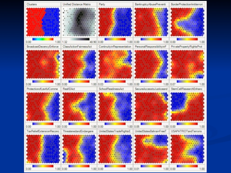
These networks widely used for clustering
SOMs (like our brain) decide the task of mapping a high-dimensional input (N dimensions) onto areas in a low-dimensional grid of cells (G dimensions).
Слайд 92Scheme of training
of self-organizing map
Слайд 93Competitive learning
Competitive learning is a form of unsupervised learning in artificial neural networks, in which
nodes compete for the right to respond to a subset of the input data
Слайд 95Vector quantization
It works by dividing a large set of points (vectors)
into groups having approximately the same number of points closest to them. Each group is represented by its centroid point, as in k-means and some other clustering algorithms.
Слайд 96Vector quantization
Choose random weights from [0;1].
t=1
Take all input patterns Xl,l=1,L
t=t+1
Applications:
data compression
pattern recognition
Video codecs
QuickTime
Cinepak
Indeo etc.
Audio codecs
Ogg Vorbis
TwinVQ
DTS etc.
Слайд 99Kohonen maps learning procedure
Choose random weights from [0;1].
t=1
Take input pattern Xl
and calculate Dij=(Xl-Wij),where i,j=1,m
Detect winner neuron D(k1,k2)=min(Dij)
Calculate for every output neuron
Modify weights by following way
Repeat steps 3-6 for all input patterns
Слайд 101Training
The goal is to achieve a balance between correct responses for
the training patterns and correct responses for new patterns.
Слайд 102Training and Verification
The set of all known samples is broken into
two independent sets
Training set
A group of samples used to train the neural network
Testing set
A group of samples used to test the performance of the neural network
Used to estimate the error rate
Слайд 103Verification
Provides an unbiased test of the quality of the network
Common
error is to “test” the neural network using the same samples that were used to train the neural network.
The network was optimized on these samples, and will obviously perform well on them
Doesn’t give any indication as to how well the network will be able to classify inputs that weren’t in the training set
Слайд 104Summary (Discussion)
Artificial neural networks are inspired by the learning processes that
take place in biological systems.
Artificial neurons and neural networks try to imitate the working mechanisms of their biological counterparts.
Learning can be perceived as an optimisation process.
Biological neural learning happens by the modification of the synaptic strength. Artificial neural networks learn in the same way.
The synapse strength modification rules for artificial neural networks can be derived by applying mathematical optimisation methods.
Слайд 105Summary
Learning tasks of artificial neural networks can be reformulated as function
approximation tasks.
Neural networks can be considered as nonlinear function approximating tools (i.e., linear combinations of nonlinear basis functions), where the parameters of the networks should be found by applying optimisation methods.
The optimisation is done with respect to the approximation error measure.
In general it is enough to have a single hidden layer neural network (MLP or other) to learn the approximation of a nonlinear function.
NEURAL")


Classification in marketing: consumer spending pattern classification In defence: radar")


The delta rule is a gradient descent learning rule for updating the weights of the inputs")
Gradient descent method: find the steepest way down the slope from where you are, and")


 based on given training patterns.")
 - a data-storage device in which a location is identified")


 is a feed forward artificial neural network model that maps sets of input data onto")


Most common method of obtaining the weights in")


3. wij=wji, wii=0")
")

Hamming network is two-network bipolar classifier. The first layer is single-layer perceptron.")


A self-organizing map (SOM) is a type of artificial neural networkA self-organizing map (SOM) is a type of artificial")


 into groups having approximately")

,where i,j=1,mDetect")


Artificial neural networks are inspired by the learning processes that take place in biological")


")
ADALINE (ADAptive LINear Element) network")


Calculation the output Y for input vector X")