- Главная
- Разное
- Дизайн
- Бизнес и предпринимательство
- Аналитика
- Образование
- Развлечения
- Красота и здоровье
- Финансы
- Государство
- Путешествия
- Спорт
- Недвижимость
- Армия
- Графика
- Культурология
- Еда и кулинария
- Лингвистика
- Английский язык
- Астрономия
- Алгебра
- Биология
- География
- Детские презентации
- Информатика
- История
- Литература
- Маркетинг
- Математика
- Медицина
- Менеджмент
- Музыка
- МХК
- Немецкий язык
- ОБЖ
- Обществознание
- Окружающий мир
- Педагогика
- Русский язык
- Технология
- Физика
- Философия
- Химия
- Шаблоны, картинки для презентаций
- Экология
- Экономика
- Юриспруденция
Introduction to CFX. Workshop 1 Mixing T-Junction презентация
Содержание
- 1. Introduction to CFX. Workshop 1 Mixing T-Junction
- 2. Welcome! This introductory tutorial models mixing of
- 3. Pre-processing Goals Launch CFX-Pre from Workbench Use
- 4. Start in Workbench The first step is
- 5. Next, expand the Component Systems toolbox and
- 6. CFX-Pre GUI Overview Outline Tree New objects
- 7. CFX-Pre Mesh and Regions A domain named
- 8. CFX-Pre – Domain settings The first step
- 9. CFX-Pre – Domain settings (continued) Double-click on
- 10. CFX-Pre – Domain settings (continued) Click the
- 11. Boundary Conditions The next step is to
- 12. CFX-Pre – Inlet boundary conditions Now that
- 13. CFX-Pre – Inlet boundary conditions (contd.) Leave
- 14. CFX-Pre – Inlet boundary conditions (contd.) This
- 15. CFX-Pre – Inlet boundary conditions (contd.) Right-click
- 16. CFX-Pre – Inlet boundary conditions (contd.) This
- 17. CFX-Pre – Outlet boundary conditions Insert a
- 18. CFX-Pre – Wall boundary conditions The default
- 19. Right-click on inlety and select Edit in
- 20. Initialisation Automatic: This will use a previous
- 21. Solver Control Double-click on Solver Control from
- 22. CFX-Pre – Monitor points Double-click Output
- 23. CFX-Pre – Monitor points (continued) An expression
- 24. CFX-Pre – Monitor points (continued) A
- 25. CFX-Pre – Monitor points (continued) An expression
- 26. Solution Goals Launch CFX-Pre from Workbench. Use
- 27. Obtaining a solution Exit CFX-Pre When running
- 28. Obtaining a solution (continued) The CFX Solver
- 29. Post-processing Goals Launch CFX-Pre from Workbench. Use
- 30. Launching CFD-Post Exit the CFX Solver Manager
- 31. CFD-Post Overview Selector Window Lists currently defined
- 32. CFD-Post – Manipulating the view When the
- 33. CFD-Post – Temperature contour plot In the
- 34. CFD-Post – Temperature contour plot (contd.) Set
- 35. CFD-Post - Temperature contour plot (contd.) A
- 36. CFD-Post Location: Points, Lines, Planes, Surfaces, Volumes
- 37. CFD-Post – Creating a plane at x
- 38. CFD-Post – Creating a plane at x
- 39. CFD-Post – Creating a velocity vector plot
- 40. CFD-Post – Velocity vector plot (continued) Set
- 41. CFD-Post – Aligning the view Given that
- 42. CFD-Post – Creating velocity streamlines Hide the
- 43. CFD-Post – Velocity streamlines (continued) In the
- 44. CFD-Post – Velocity streamlines (continued) Click the
- 45. CFD-Post – Creating a velocity isosurface Hide
- 46. CFD-Post – Velocity isosurface (continued) Set the
- 47. CFD-Post – Velocity isosurface (continued) By default,
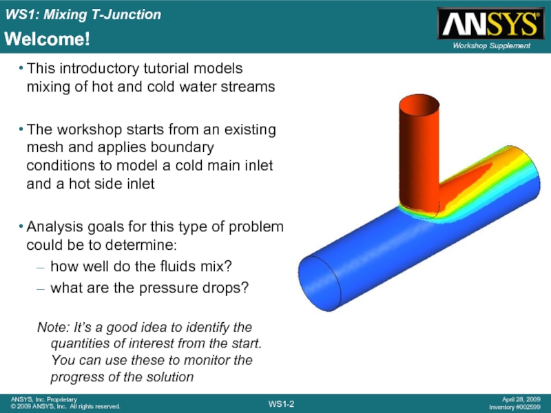
Слайд 2Welcome!
This introductory tutorial models mixing of hot and cold water streams
The
Analysis goals for this type of problem could be to determine:
how well do the fluids mix?
what are the pressure drops?
Note: It’s a good idea to identify the quantities of interest from the start. You can use these to monitor the progress of the solution
Слайд 3Pre-processing Goals
Launch CFX-Pre from Workbench
Use pre-defined materials
Define the fluid models in
Create and edit objects in CFX-Pre
Define boundary conditions
Set up monitor points using simple expressions
Launch CFD-Post from an existing CFX simulation in Workbench
Rotate, zoom and pan the view
Create contour plots
Create a plane for use as a locator
Create a velocity vector plot
Use pre-defined views
Create streamlines of velocity
Create an isosurface, coloured by a separate variable
Launch the CFX Solver Manager from Workbench
Monitor convergence
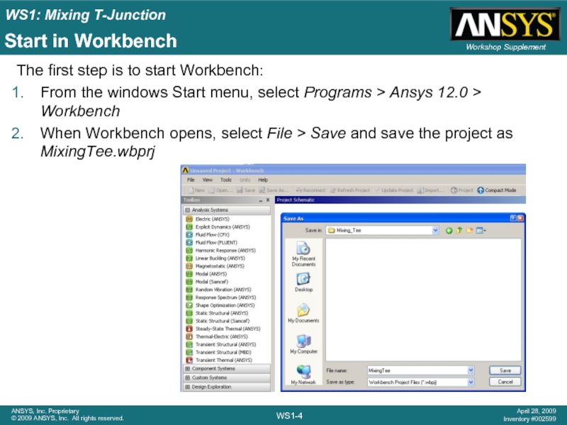
Слайд 4Start in Workbench
The first step is to start Workbench:
From the windows
When Workbench opens, select File > Save and save the project as MixingTee.wbprj
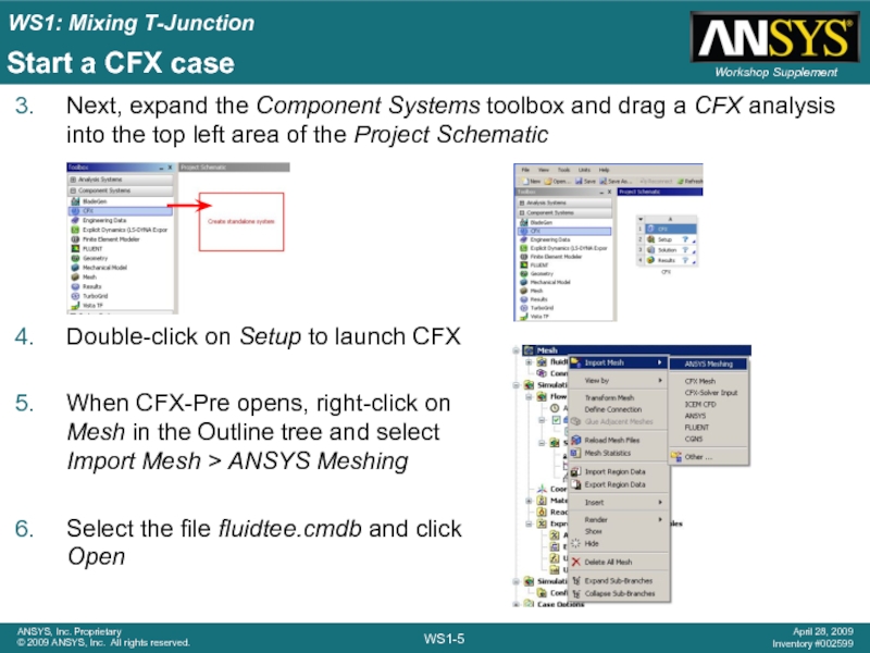
Слайд 5Next, expand the Component Systems toolbox and drag a CFX analysis
Double-click on Setup to launch CFX
When CFX-Pre opens, right-click on Mesh in the Outline tree and select Import Mesh > ANSYS Meshing
Select the file fluidtee.cmdb and click Open
Start a CFX case
Слайд 6CFX-Pre GUI Overview
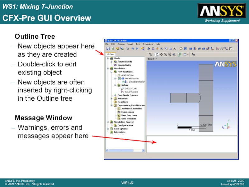
Outline Tree
New objects appear here as they are created
Double-click
New objects are often inserted by right-clicking in the Outline tree
Message Window
Warnings, errors and messages appear here
Слайд 7CFX-Pre Mesh and Regions
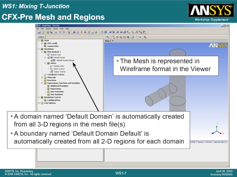
A domain named ‘Default Domain’ is automatically created
A boundary named ‘Default Domain Default’ is automatically created from all 2-D regions for each domain
The Mesh is represented in Wireframe format in the Viewer
Слайд 8CFX-Pre – Domain settings
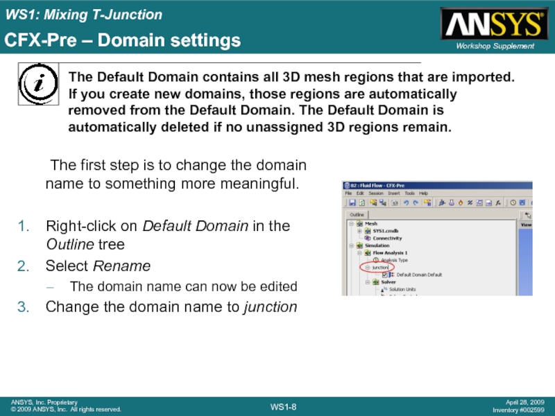
The first step is to change the domain
Right-click on Default Domain in the Outline tree
Select Rename
The domain name can now be edited
Change the domain name to junction
Слайд 9CFX-Pre – Domain settings (continued)
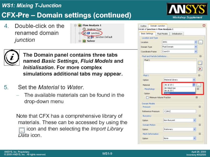
Double-click on the renamed domain junction
Set the
The available materials can be found in the drop-down menu
Note that CFX has a comprehensive library of materials. These can be accessed by using the icon and then selecting the Import Library Data icon.
Слайд 10CFX-Pre – Domain settings (continued)
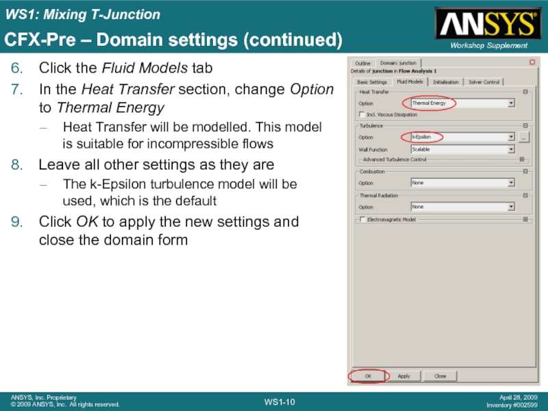
Click the Fluid Models tab
In the Heat
Heat Transfer will be modelled. This model is suitable for incompressible flows
Leave all other settings as they are
The k-Epsilon turbulence model will be used, which is the default
Click OK to apply the new settings and close the domain form
Слайд 11Boundary Conditions
The next step is to create the boundary conditions. You
Слайд 12CFX-Pre – Inlet boundary conditions
Now that the domain exists, boundary conditions
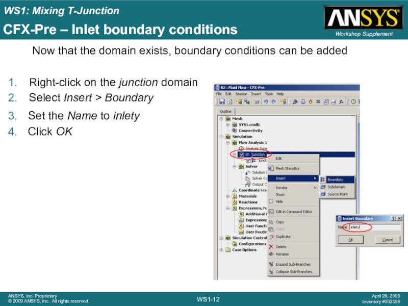
Right-click on the junction domain
Select Insert > Boundary
Set the Name to inlety
Click OK
Слайд 13CFX-Pre – Inlet boundary conditions (contd.)
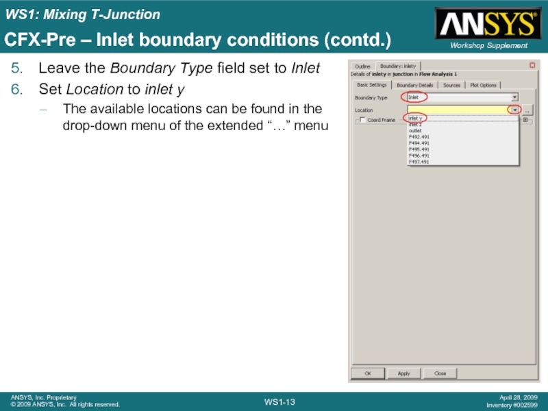
Leave the Boundary Type field set
Set Location to inlet y
The available locations can be found in the drop-down menu of the extended “…” menu
Слайд 14CFX-Pre – Inlet boundary conditions (contd.)
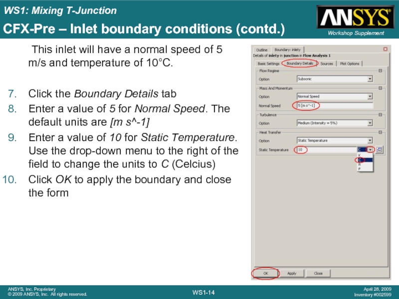
This inlet will have a normal
Click the Boundary Details tab
Enter a value of 5 for Normal Speed. The default units are [m s^-1]
Enter a value of 10 for Static Temperature. Use the drop-down menu to the right of the field to change the units to C (Celcius)
Click OK to apply the boundary and close the form
Слайд 15CFX-Pre – Inlet boundary conditions (contd.)
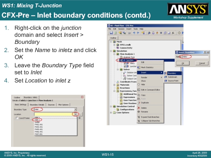
Right-click on the junction domain and
Set the Name to inletz and click OK
Leave the Boundary Type field set to Inlet
Set Location to inlet z
Слайд 16CFX-Pre – Inlet boundary conditions (contd.)
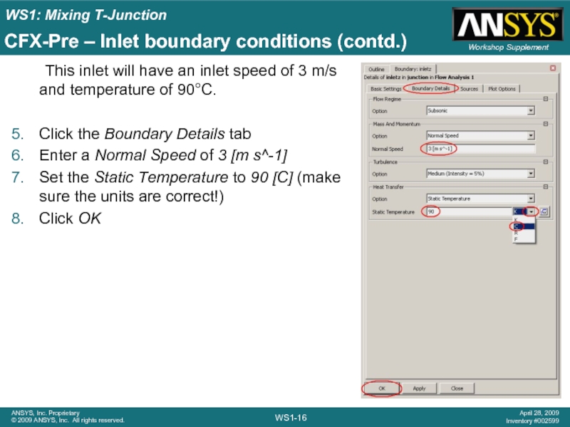
This inlet will have an inlet
Click the Boundary Details tab
Enter a Normal Speed of 3 [m s^-1]
Set the Static Temperature to 90 [C] (make sure the units are correct!)
Click OK
Слайд 17CFX-Pre – Outlet boundary conditions
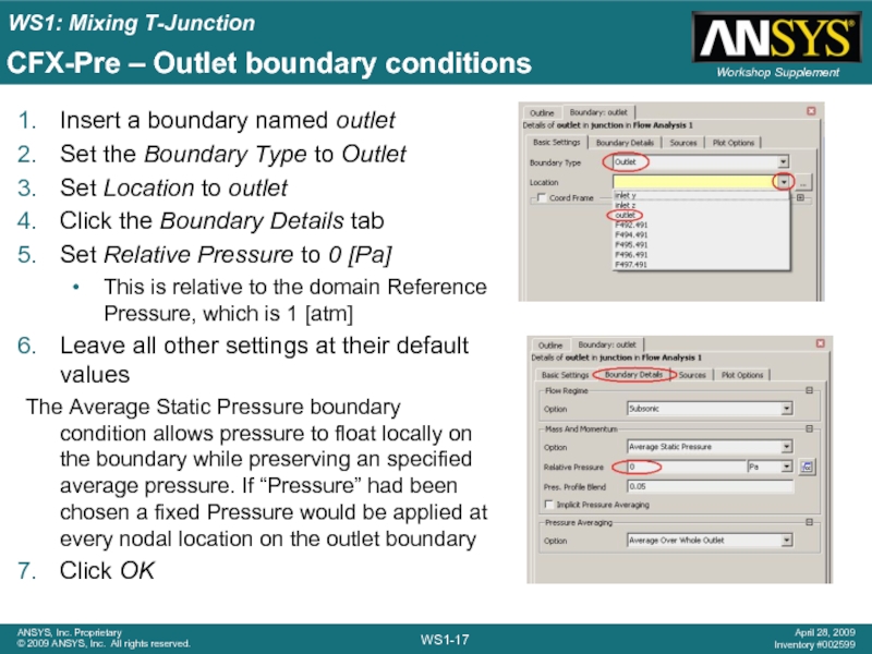
Insert a boundary named outlet
Set the Boundary
Set Location to outlet
Click the Boundary Details tab
Set Relative Pressure to 0 [Pa]
This is relative to the domain Reference Pressure, which is 1 [atm]
Leave all other settings at their default values
The Average Static Pressure boundary condition allows pressure to float locally on the boundary while preserving an specified average pressure. If “Pressure” had been chosen a fixed Pressure would be applied at every nodal location on the outlet boundary
Click OK
Слайд 18CFX-Pre – Wall boundary conditions
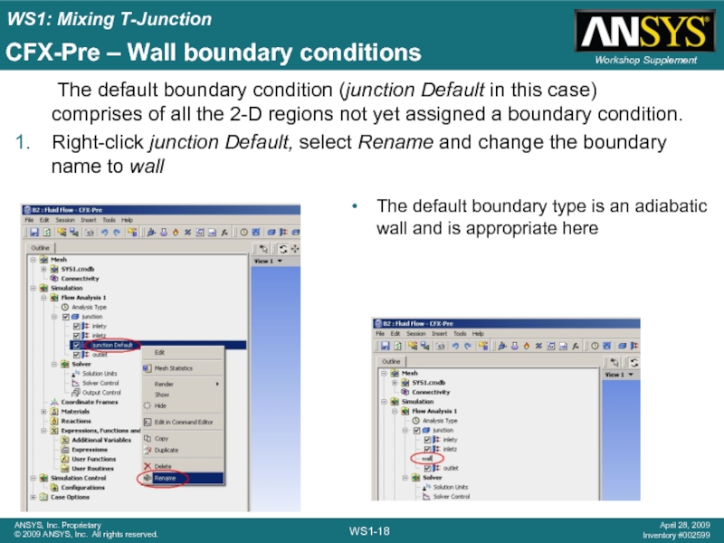
The default boundary condition (junction Default in
Right-click junction Default, select Rename and change the boundary name to wall
The default boundary type is an adiabatic wall and is appropriate here
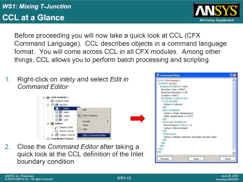
Слайд 19Right-click on inlety and select Edit in Command Editor
Close the Command
CCL at a Glance
Before proceeding you will now take a quick look at CCL (CFX Command Language). CCL describes objects in a command language format. You will come across CCL in all CFX modules. Among other things, CCL allows you to perform batch processing and scripting.
Слайд 20Initialisation
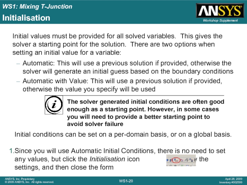
Automatic: This will use a previous solution if provided, otherwise the
Automatic with Value: This will use a previous solution if provided, otherwise the value you specify will be used
Initial values must be provided for all solved variables. This gives the solver a starting point for the solution. There are two options when setting an initial value for a variable:
Initial conditions can be set on a per-domain basis, or on a global basis.
Since you will use Automatic Initial Conditions, there is no need to set any values, but click the Initialisation icon to view the settings, and then close the form
Слайд 21Solver Control
Double-click on Solver Control from the Outline tree
The solver will
Advection Scheme and Timescale Control will be discussed later
Residuals are a measure of how well the posed equations have been solved. In this case the solver will stop when the RMS (Root Mean Squared) residuals have reached 1.E-4. Tighter convergence is achieved with lower residuals.
Click Close
The Solver Control options set various parameters that are used by the solver and can affect the accuracy of the results. The default settings are reasonable, but will not be correct for all simulations. In this case the default settings will be used, but you will still look at what those defaults are.
Слайд 22CFX-Pre – Monitor points
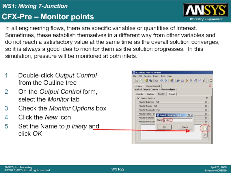
Double-click Output Control from the Outline tree
On the
Check the Monitor Options box
Click the New icon
Set the Name to p inlety and click OK
In all engineering flows, there are specific variables or quantities of interest. Sometimes, these establish themselves in a different way from other variables and do not reach a satisfactory value at the same time as the overall solution converges, so it is always a good idea to monitor them as the solution progresses. In this simulation, pressure will be monitored at both inlets.
Слайд 23CFX-Pre – Monitor points (continued)
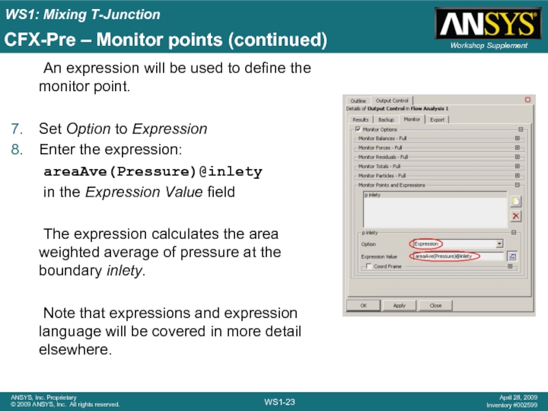
An expression will be used to define
Set Option to Expression
Enter the expression:
areaAve(Pressure)@inlety
in the Expression Value field
The expression calculates the area weighted average of pressure at the boundary inlety.
Note that expressions and expression language will be covered in more detail elsewhere.
Слайд 24CFX-Pre – Monitor points (continued)
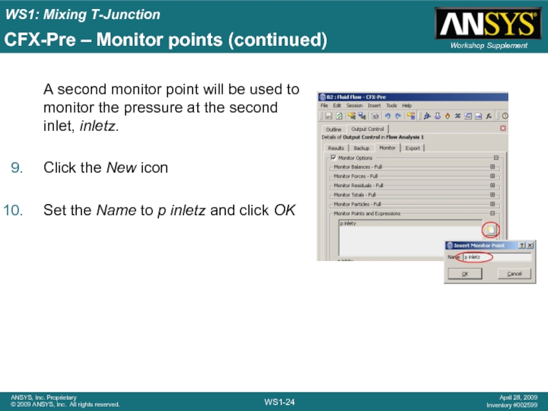
A second monitor point will be used
Click the New icon
Set the Name to p inletz and click OK
Слайд 25CFX-Pre – Monitor points (continued)
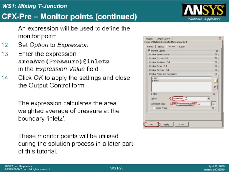
An expression will be used to define
Set Option to Expression
Enter the expression areaAve(Pressure)@inletz in the Expression Value field
Click OK to apply the settings and close the Output Control form
The expression calculates the area weighted average of pressure at the boundary ‘inletz’.
These monitor points will be utilised during the solution process in a later part of this tutorial.
Слайд 26Solution Goals
Launch CFX-Pre from Workbench.
Use pre-defined materials.
Define the fluid models in
Create and edit objects in CFX-Pre.
Define boundary conditions.
Set up monitor points using simple expressions.
Launch CFD-Post from an existing CFX Simulation in Workbench.
Rotate, zoom and pan the view.
Create contour plots.
Create a plane for use as a locator.
Create a velocity vector plot.
Use pre-defined views.
Create streamlines of velocity.
Create an isosurface, coloured by a separate variable.
Launch the CFX Solver Manager from Workbench.
Monitor convergence.
Слайд 27Obtaining a solution
Exit CFX-Pre
When running in WB the CFX-Pre case will
Save the Workbench project
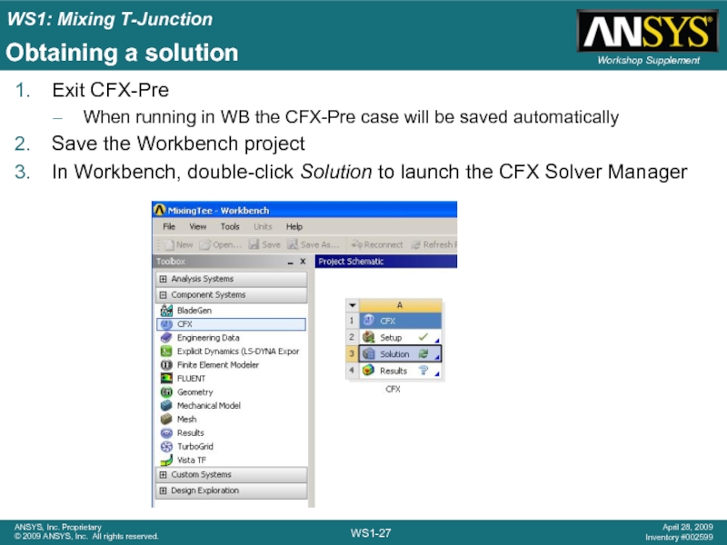
In Workbench, double-click Solution to launch the CFX Solver Manager
Слайд 28Obtaining a solution (continued)
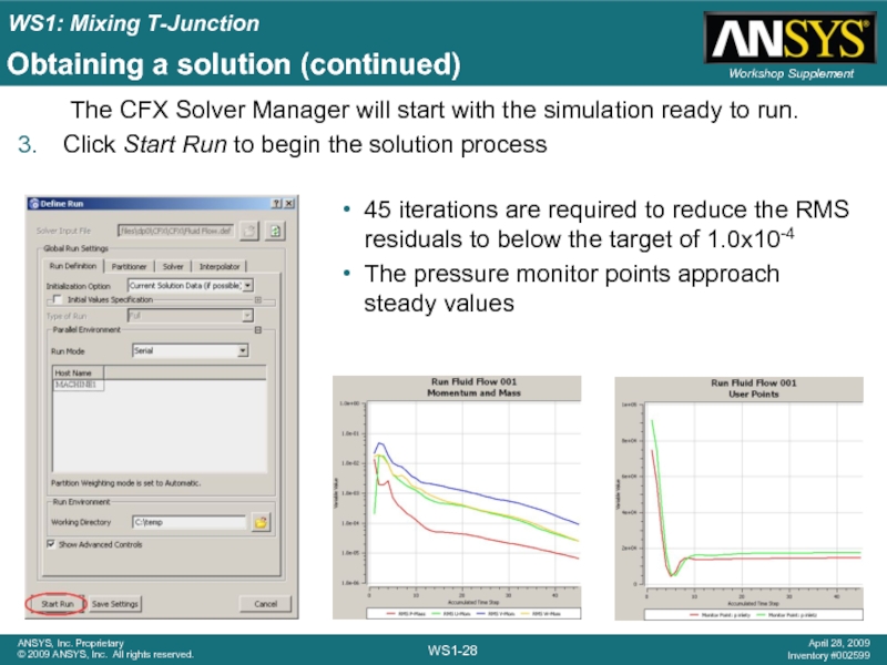
The CFX Solver Manager will start with the
Click Start Run to begin the solution process
45 iterations are required to reduce the RMS residuals to below the target of 1.0x10⁻⁴
The pressure monitor points approach steady values
Слайд 29Post-processing Goals
Launch CFX-Pre from Workbench.
Use pre-defined materials.
Define the fluid models in
Create and edit objects in CFX-Pre.
Define boundary conditions.
Set up monitor points using simple expressions.
Launch CFD-Post from an existing CFX Simulation in Workbench.
Rotate, zoom and pan the view.
Create contour plots.
Create a plane for use as a locator.
Create a velocity vector plot.
Use pre-defined views.
Create streamlines of velocity.
Create an isosurface, coloured by a separate variable.
Launch the CFX solver manager from Workbench.
Monitor convergence.
Слайд 30Launching CFD-Post
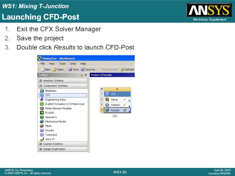
Exit the CFX Solver Manager
Save the project
Double click Results to
Слайд 31CFD-Post Overview
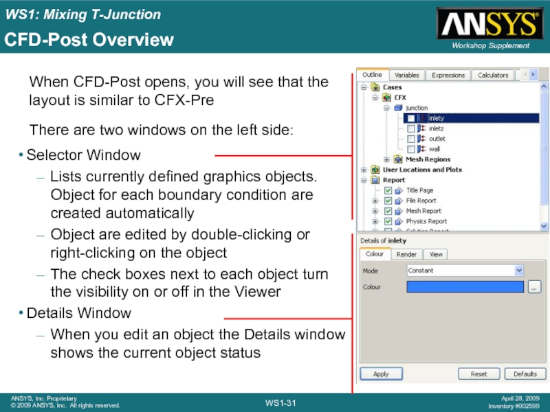
Selector Window
Lists currently defined graphics objects. Object for each boundary
Object are edited by double-clicking or right-clicking on the object
The check boxes next to each object turn the visibility on or off in the Viewer
Details Window
When you edit an object the Details window shows the current object status
When CFD-Post opens, you will see that the layout is similar to CFX-Pre
There are two windows on the left side:
Слайд 32CFD-Post – Manipulating the view
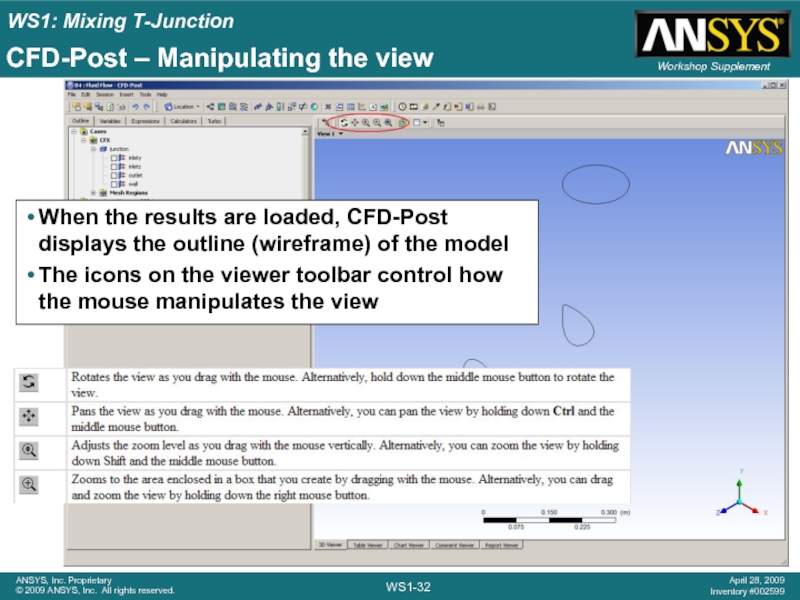
When the results are loaded, CFD-Post displays
The icons on the viewer toolbar control how the mouse manipulates the view
Слайд 33CFD-Post – Temperature contour plot
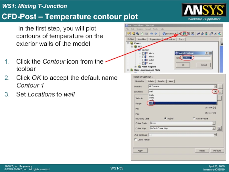
In the first step, you will plot
Click the Contour icon from the toolbar
Click OK to accept the default name Contour 1
Set Locations to wall
Слайд 34CFD-Post – Temperature contour plot (contd.)
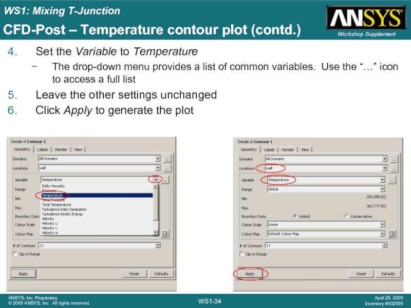
Set the Variable to Temperature
The drop-down
Leave the other settings unchanged
Click Apply to generate the plot
Слайд 35CFD-Post - Temperature contour plot (contd.)
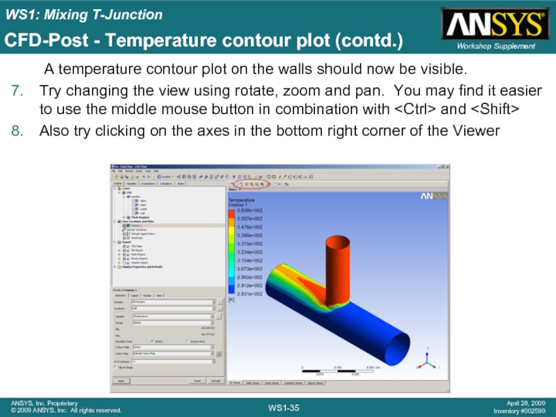
A temperature contour plot on the
Try changing the view using rotate, zoom and pan. You may find it easier to use the middle mouse button in combination with
Also try clicking on the axes in the bottom right corner of the Viewer
Слайд 36CFD-Post
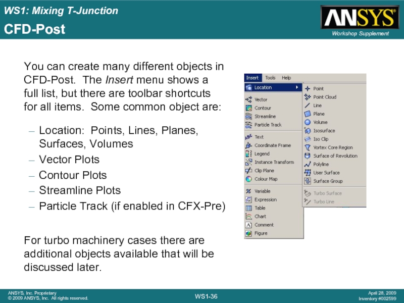
Location: Points, Lines, Planes, Surfaces, Volumes
Vector Plots
Contour Plots
Streamline Plots
Particle Track (if
You can create many different objects in CFD-Post. The Insert menu shows a full list, but there are toolbar shortcuts for all items. Some common object are:
For turbo machinery cases there are additional objects available that will be discussed later.
Слайд 37CFD-Post – Creating a plane at x = 0
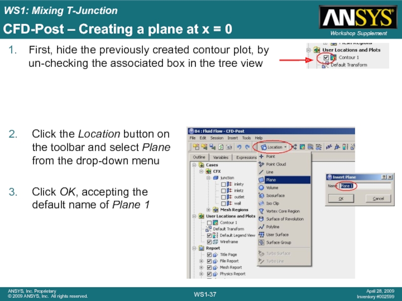
First, hide the
Click the Location button on the toolbar and select Plane from the drop-down menu
Click OK, accepting the default name of Plane 1
Слайд 38CFD-Post – Creating a plane at x = 0 (contd.)
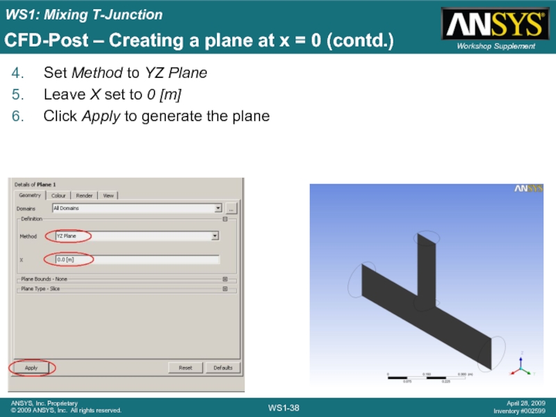
Set Method
Leave X set to 0 [m]
Click Apply to generate the plane
Слайд 39CFD-Post – Creating a velocity vector plot
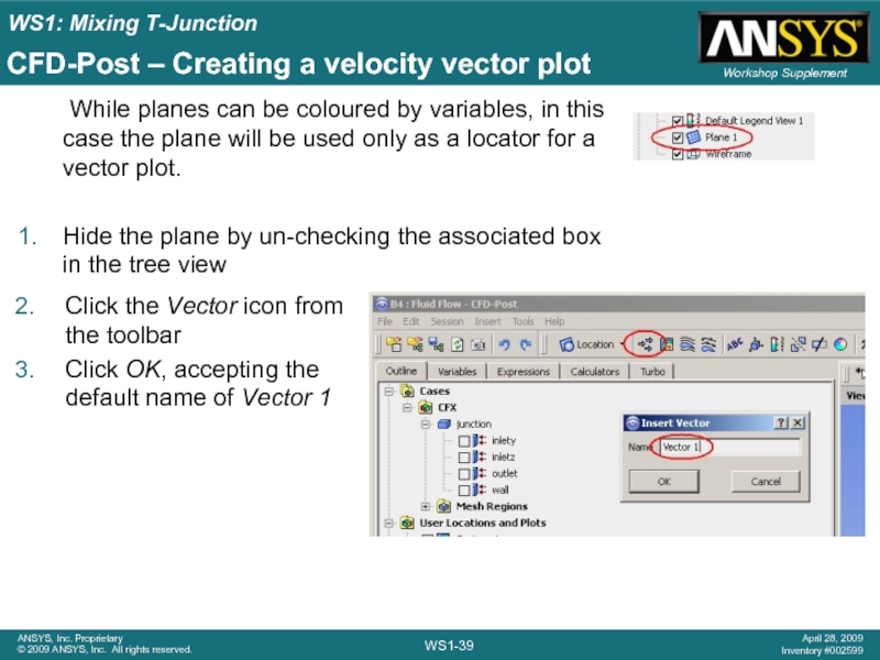
While planes can be coloured
Hide the plane by un-checking the associated box in the tree view
Click the Vector icon from the toolbar
Click OK, accepting the default name of Vector 1
Слайд 40CFD-Post – Velocity vector plot (continued)
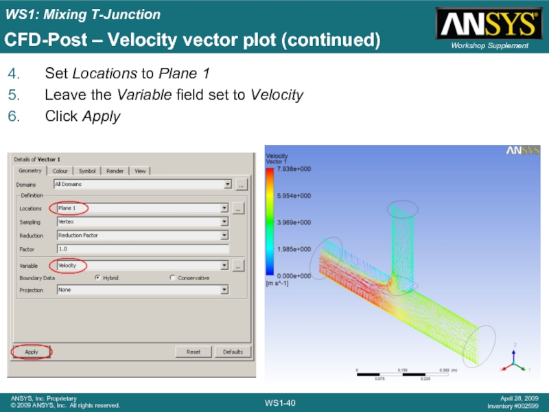
Set Locations to Plane 1
Leave the
Click Apply
Слайд 41CFD-Post – Aligning the view
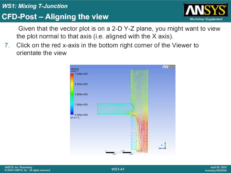
Given that the vector plot is on
Click on the red x-axis in the bottom right corner of the Viewer to orientate the view
Слайд 42CFD-Post – Creating velocity streamlines
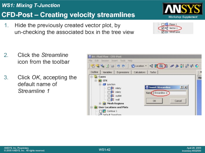
Hide the previously created vector plot, by
Click the Streamline icon from the toolbar
Click OK, accepting the default name of Streamline 1
Слайд 43CFD-Post – Velocity streamlines (continued)
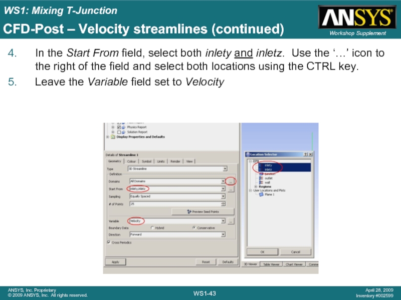
In the Start From field, select both
Leave the Variable field set to Velocity
Слайд 44CFD-Post – Velocity streamlines (continued)
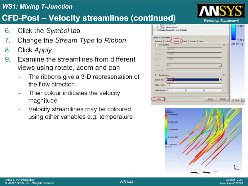
Click the Symbol tab
Change the Stream Type
Click Apply
Examine the streamlines from different views using rotate, zoom and pan
The ribbons give a 3-D representation of the flow direction
Their colour indicates the velocity magnitude
Velocity streamlines may be coloured using other variables e.g. temperature
Слайд 45CFD-Post – Creating a velocity isosurface
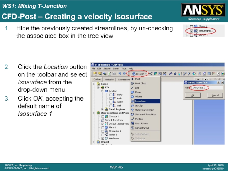
Hide the previously created streamlines, by
Click the Location button on the toolbar and select Isosurface from the drop-down menu
Click OK, accepting the default name of Isosurface 1
Слайд 46CFD-Post – Velocity isosurface (continued)
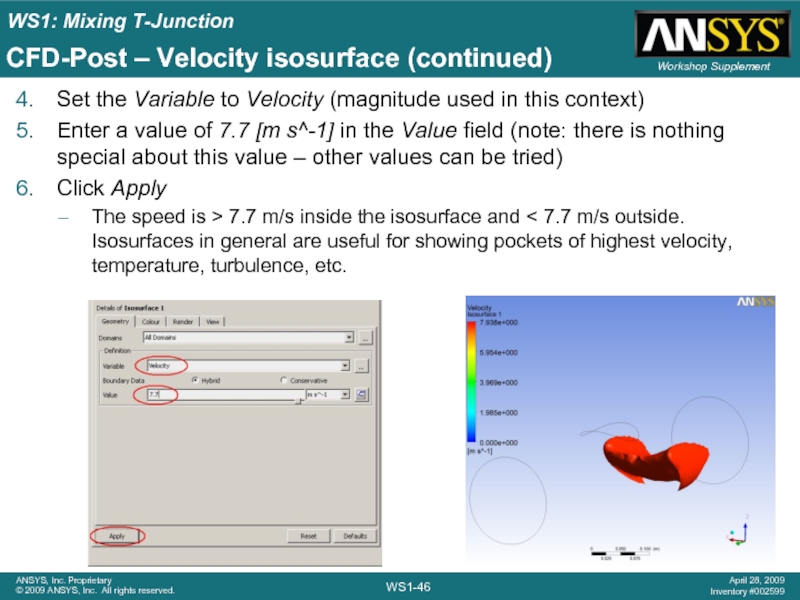
Set the Variable to Velocity (magnitude used
Enter a value of 7.7 [m s^-1] in the Value field (note: there is nothing special about this value – other values can be tried)
Click Apply
The speed is > 7.7 m/s inside the isosurface and < 7.7 m/s outside. Isosurfaces in general are useful for showing pockets of highest velocity, temperature, turbulence, etc.
Слайд 47CFD-Post – Velocity isosurface (continued)
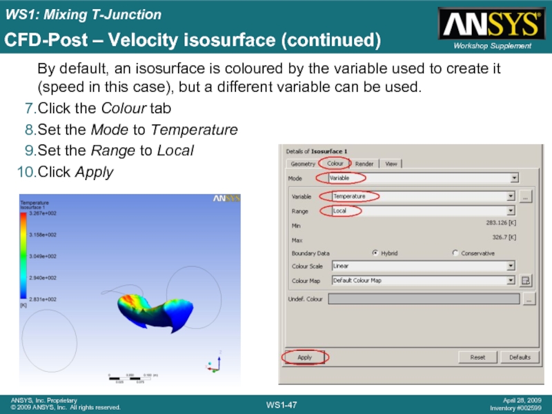
By default, an isosurface is coloured by
Click the Colour tab
Set the Mode to Temperature
Set the Range to Local
Click Apply

