- Главная
- Разное
- Дизайн
- Бизнес и предпринимательство
- Аналитика
- Образование
- Развлечения
- Красота и здоровье
- Финансы
- Государство
- Путешествия
- Спорт
- Недвижимость
- Армия
- Графика
- Культурология
- Еда и кулинария
- Лингвистика
- Английский язык
- Астрономия
- Алгебра
- Биология
- География
- Детские презентации
- Информатика
- История
- Литература
- Маркетинг
- Математика
- Медицина
- Менеджмент
- Музыка
- МХК
- Немецкий язык
- ОБЖ
- Обществознание
- Окружающий мир
- Педагогика
- Русский язык
- Технология
- Физика
- Философия
- Химия
- Шаблоны, картинки для презентаций
- Экология
- Экономика
- Юриспруденция
Introduction to artificial intelligence А* Search презентация
Содержание
- 1. Introduction to artificial intelligence А* Search
- 2. Best-First Search Review Advantages Takes advantage of
- 3. The A* Algorithm Consider the overall cost
- 4. The A* Algorithm A*-Search(initial-test)
- 5. A* Search: Example Travel: h(n) = distance(n,
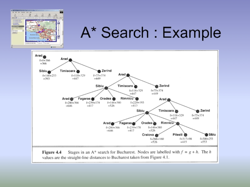
- 6. A* Search : Example
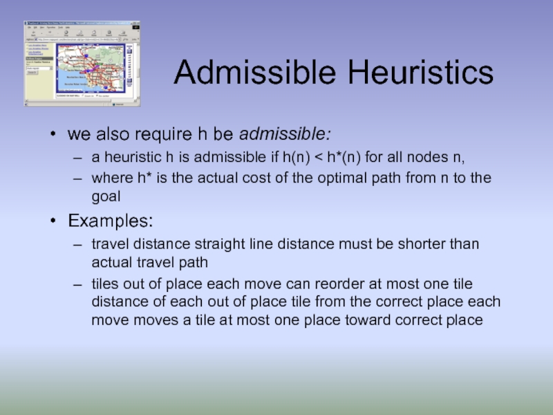
- 7. Admissible Heuristics we also require h be
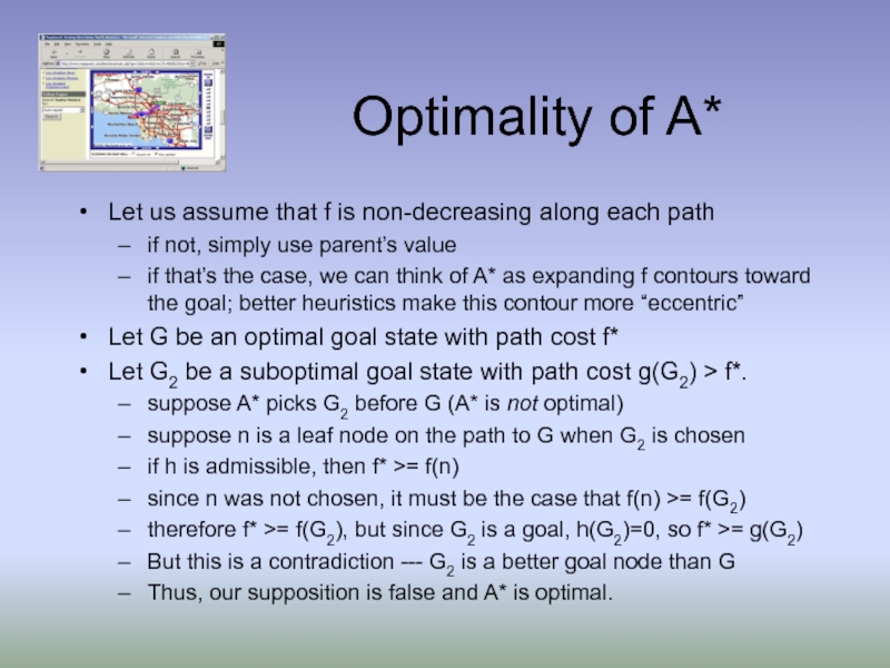
- 8. Optimality of A* Let us assume that
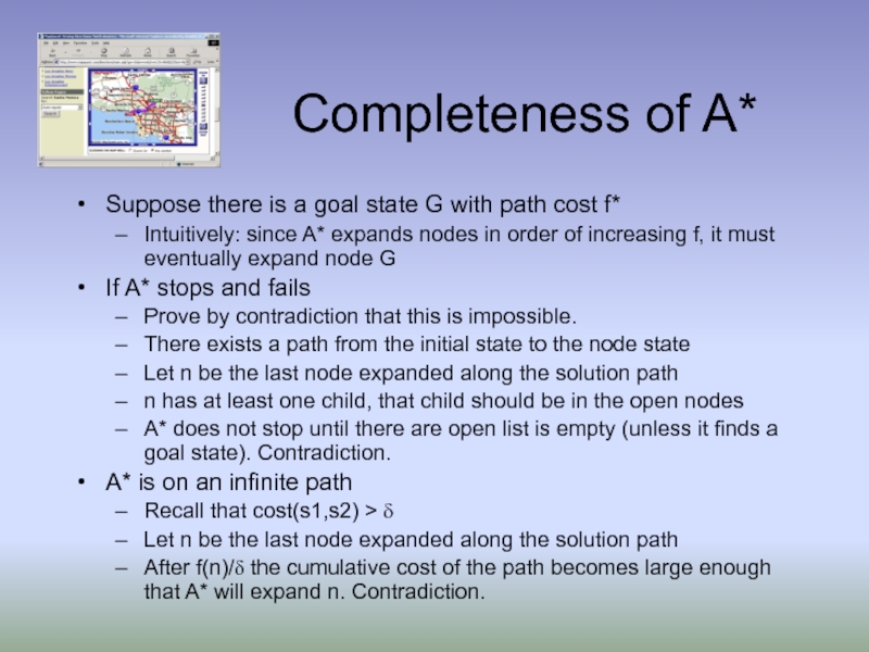
- 9. Completeness of A* Suppose there is a
- 10. UCS, BFS, Best-First, and A* f =
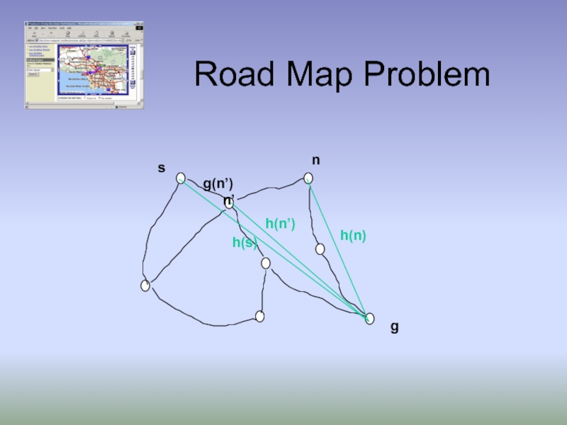
- 11. Road Map Problem
- 12. 8-queens State contains 8 queens on the
- 13. Heuristics : 8 Puzzle
- 14. 8 Puzzle Reachable state : 9!/2 =
- 15. Effect of Heuristic Accuracy on Performance Well-designed
- 17. A* summary Completeness provided finite branching
- 18. Relax Optimality Goals: Minimizing search cost Satisficing
- 19. Iterative Deepening A* Goals A storage efficient
- 20. IDA* Algorithm IDA* (state,h) returns solution f-limit
- 21. IDA* Properties Complete: if shortest path fits
- 22. Mapquest http://www.mapquest.com/ MapQuest uses a "double Dijkstra"
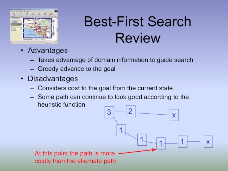
Слайд 2Best-First Search Review
Advantages
Takes advantage of domain information to guide search
Greedy advance
Disadvantages
Considers cost to the goal from the current state
Some path can continue to look good according to the heuristic function
At this point the path is more
costly than the alternate path
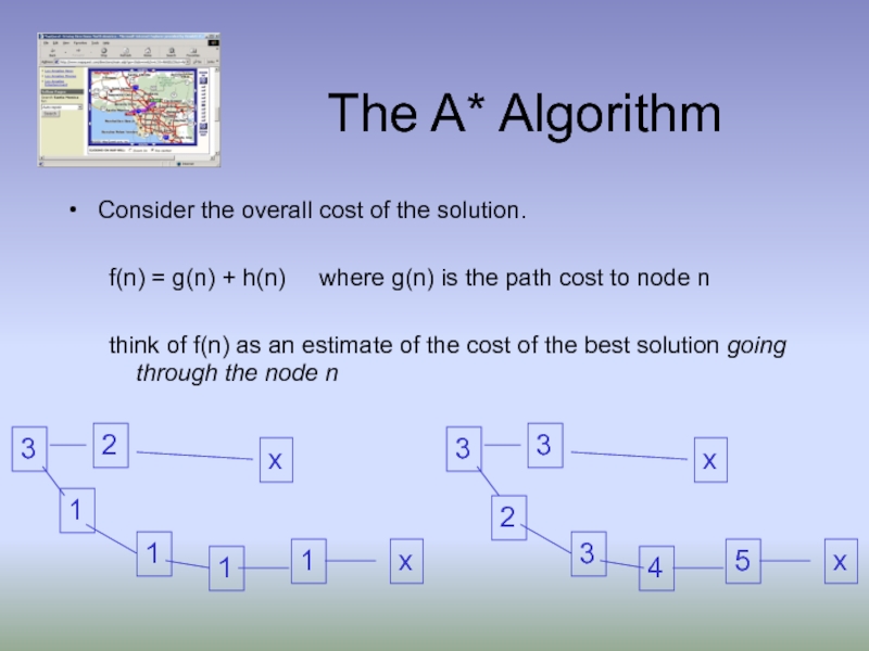
Слайд 3The A* Algorithm
Consider the overall cost of the solution.
f(n) =
think of f(n) as an estimate of the cost of the best solution going through the node n
3
3
2
x
3
4
5
x
3
2
1
x
1
1
1
x
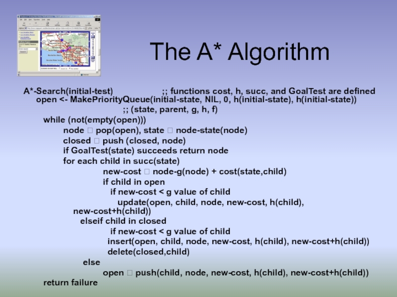
Слайд 4The A* Algorithm
A*-Search(initial-test)
;; (state, parent, g, h, f)
while (not(empty(open)))
node ? pop(open), state ? node-state(node)
closed ? push (closed, node)
if GoalTest(state) succeeds return node
for each child in succ(state)
new-cost ? node-g(node) + cost(state,child)
if child in open
if new-cost < g value of child
update(open, child, node, new-cost, h(child), new-cost+h(child))
elseif child in closed
if new-cost < g value of child
insert(open, child, node, new-cost, h(child), new-cost+h(child))
delete(closed,child)
else
open ? push(child, node, new-cost, h(child), new-cost+h(child))
return failure
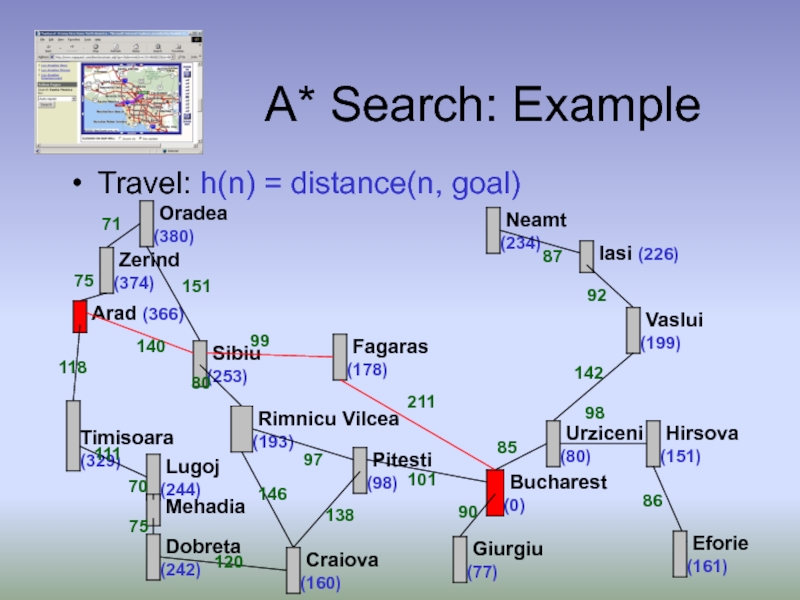
Слайд 5A* Search: Example
Travel: h(n) = distance(n, goal)
71
142
85
90
101
97
99
140
138
146
120
75
70
111
118
75
211
151
86
98
92
87
80
Слайд 7Admissible Heuristics
we also require h be admissible:
a heuristic h is
where h* is the actual cost of the optimal path from n to the goal
Examples:
travel distance straight line distance must be shorter than actual travel path
tiles out of place each move can reorder at most one tile distance of each out of place tile from the correct place each move moves a tile at most one place toward correct place
Слайд 8Optimality of A*
Let us assume that f is non-decreasing along each
if not, simply use parent’s value
if that’s the case, we can think of A* as expanding f contours toward the goal; better heuristics make this contour more “eccentric”
Let G be an optimal goal state with path cost f*
Let G2 be a suboptimal goal state with path cost g(G2) > f*.
suppose A* picks G2 before G (A* is not optimal)
suppose n is a leaf node on the path to G when G2 is chosen
if h is admissible, then f* >= f(n)
since n was not chosen, it must be the case that f(n) >= f(G2)
therefore f* >= f(G2), but since G2 is a goal, h(G2)=0, so f* >= g(G2)
But this is a contradiction --- G2 is a better goal node than G
Thus, our supposition is false and A* is optimal.
Слайд 9Completeness of A*
Suppose there is a goal state G with path
Intuitively: since A* expands nodes in order of increasing f, it must eventually expand node G
If A* stops and fails
Prove by contradiction that this is impossible.
There exists a path from the initial state to the node state
Let n be the last node expanded along the solution path
n has at least one child, that child should be in the open nodes
A* does not stop until there are open list is empty (unless it finds a goal state). Contradiction.
A* is on an infinite path
Recall that cost(s1,s2) > δ
Let n be the last node expanded along the solution path
After f(n)/δ the cumulative cost of the path becomes large enough that A* will expand n. Contradiction.
Слайд 10UCS, BFS, Best-First, and A*
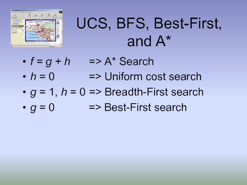
f = g + h
h = 0 => Uniform cost search
g = 1, h = 0 => Breadth-First search
g = 0 => Best-First search
Слайд 128-queens
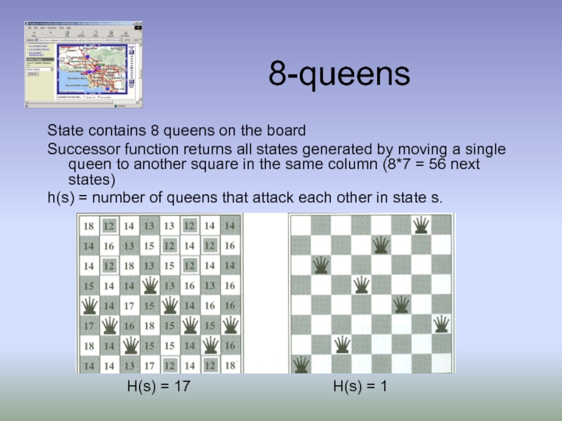
State contains 8 queens on the board
Successor function returns all states
h(s) = number of queens that attack each other in state s.
H(s) = 17
H(s) = 1
Слайд 148 Puzzle
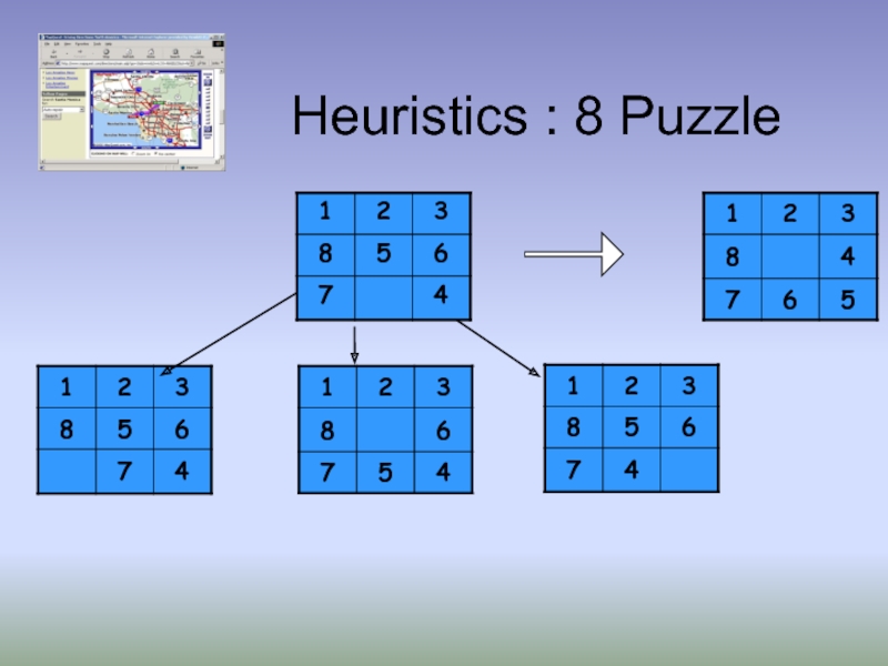
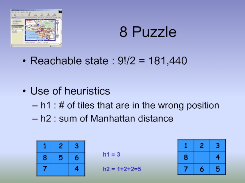
Reachable state : 9!/2 = 181,440
Use of heuristics
h1 :
h2 : sum of Manhattan distance
h1 = 3
h2 = 1+2+2=5
Слайд 15Effect of Heuristic Accuracy on Performance
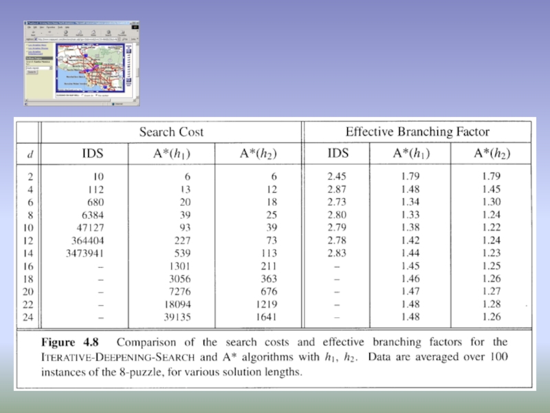
Well-designed heuristic have its branch close
h2 dominates h1 iff
h2(n) ≥ h1(n), ∀ n
It is always better to use a heuristic function with higher values, as long as it does not overestimate
Inventing heuristic functions
Cost of an exact solution to a relaxed problem is a good heuristic for the original problem
collection of admissible heuristics
h*(n) = max(h1(n), h2(n), …, hk(n))
Слайд 17A* summary
Completeness
provided finite branching factor and finite cost per operator
Optimality
provided we use an admissible heuristic
Time complexity
worst case is still O(bd) in some special cases we can do better for a given heuristic
Space complexity
worst case is still O(bd)
Слайд 18Relax Optimality
Goals:
Minimizing search cost
Satisficing solution, i.e. bounded error in the solution
f(s)
g can be thought of as the breadth first component
w = 1 => Best-First search
w = .5 => A* search
w = 0 => Uniform search
Слайд 19Iterative Deepening A*
Goals
A storage efficient algorithm that we can use in
Still complete and optimal
Modification of A*
use f-cost limit as depth bound
increase threshold as minimum of f(.) of previous cycle
Each iteration expands all nodes inside the contour for current f-cost
same order of node expansion
Слайд 20IDA* Algorithm
IDA* (state,h) returns solution
f-limit
if solution is non-null return solution
if f-limit = ∞ return failure
end
DFS-Contour (node,f-limit) returns solution
if f (node) > f-limit return null, f(node)
if GoalTest(node) return node, f-limit
next-f ? ∞
for each node s in succ(node) do
solution, new-f ? DFS-Contour(s, f-limit)
if solution is non-null return solution, f-limit
next-f ? Min(next-f, new-f)
end
return null, next-f
Слайд 21IDA* Properties
Complete:
if shortest path fits into memory
Optimal:
if shortest optimal path fits
Time Complexity: O(b2d)
Space Complexity: O(bd)
Слайд 22Mapquest
http://www.mapquest.com/
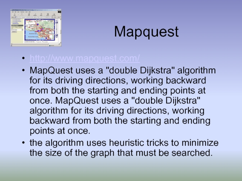
MapQuest uses a "double Dijkstra" algorithm for its driving directions, working
the algorithm uses heuristic tricks to minimize the size of the graph that must be searched.
