- Главная
- Разное
- Дизайн
- Бизнес и предпринимательство
- Аналитика
- Образование
- Развлечения
- Красота и здоровье
- Финансы
- Государство
- Путешествия
- Спорт
- Недвижимость
- Армия
- Графика
- Культурология
- Еда и кулинария
- Лингвистика
- Английский язык
- Астрономия
- Алгебра
- Биология
- География
- Детские презентации
- Информатика
- История
- Литература
- Маркетинг
- Математика
- Медицина
- Менеджмент
- Музыка
- МХК
- Немецкий язык
- ОБЖ
- Обществознание
- Окружающий мир
- Педагогика
- Русский язык
- Технология
- Физика
- Философия
- Химия
- Шаблоны, картинки для презентаций
- Экология
- Экономика
- Юриспруденция
Fault-Tolerant Design презентация
Содержание
- 1. Fault-Tolerant Design
- 2. What is this chapter about? Gives Overview
- 3. Fault-Tolerant Design Introduction Fundamentals of Fault Tolerance
- 4. Introduction Fault Tolerance Ability of system to
- 5. Faults Permanent Faults Due to manufacturing defects,
- 6. Temporary Faults Transient Errors (Non-recurring errors) Cause
- 7. Redundancy Fault Tolerance requires some form of redundancy Time Redundancy Hardware Redundancy Information Redundancy
- 8. Time Redundancy Perform Same Operation Twice See
- 9. Hardware Redundancy Replicate hardware and compare outputs
- 10. Information Redundancy Encode outputs with error detecting
- 11. Failure Rate λ(t) = Component failure rate Measured in FITS (failures per 109 hours)
- 12. System Failure Rate System constructed from components
- 13. Reliability If component working at time 0
- 14. Reliability for Series System Series System All
- 15. System Reliability with Redundancy System reliability with
- 16. Mean-Time-to-Failure (MTTF) Average time before system fails
- 17. Maintainability If system failed at time 0
- 18. Repair Rate and MTTR μ = rate
- 19. Availability System Availability Fraction of time system is operational
- 20. Availability Telephone Systems Required to have system
- 21. Coding Theory Coding Using more bits than
- 22. Block Code Message = Data Being Encoded
- 23. Block Code To detect errors, some redundancy
- 24. Separable Block Code Separable n-bit blocks partitioned
- 25. Example of Separable Block Code (4,3) Parity
- 26. Example of Non-Separable Block Code One-Hot Code
- 27. Linear Block Codes Special class Modulo-2 sum
- 28. Linear Block Codes Generator Matrix, G kxn
- 29. Systematic Block Code First k-bits correspond to
- 30. Distance of Code Distance between two codewords
- 31. Error Correcting Codes Code with distance 3
- 32. Hamming Code For any value of n
- 33. Error Correction in Hamming Code Syndrome, s
- 34. Example of Error Correction For (7,3) Hamming
- 35. SEC-DED Code Make SEC Hamming Code SEC-DED
- 36. Example of Error Correction For (7,4) SEC-DED
- 37. Hsiao Code Weight of column Number of
- 38. Example of Hsiao Code (7,3) Hsiao Code Uses weight-1 and weight-3 columns
- 39. Unidirectional Errors Errors in block of data
- 40. Unidirectional Error Detecting Codes All unidirectional error
- 41. Two-Rail Code Two-Rail Code One check bit
- 42. Berger Codes Lowest redundancy of separable AUED
- 43. Berger Codes Codewords for (5,3) Berger Code
- 44. Berger Codes If 8 information bits Berger
- 45. Constant Weight Codes Constant Weight Codes Non-separable,
- 46. Constant Weight Codes Number codewords in m-out-of-n
- 47. Example 6-out-of-12 constant weight code
- 48. Constant Weight Codes Advantage Less redundancy than
- 49. Burst Error Burst Error Common, multi-bit errors
- 50. Cyclic Codes Special class of linear code
- 51. Cyclic Redundancy Check (CRC) Code Most widely
- 53. CRC Code Linear block code Has G-matrix
- 54. CRC Code Example (6,4) CRC code generated by g(x)=x2+1
- 55. Systematic CRC Codes To obtain systematic CRC
- 56. Galois Division Example Encode m(x)=x2+x with g(x)=x2+1
- 58. Generating Check Bits for CRC Code Use
- 59. Checking CRC Codeword Checking Received Codeword for
- 60. Selecting Generator Polynomial Key issue for CRC
- 61. Commonly Used CRC Generators
- 62. Fault Tolerance Schemes Adding Fault Tolerance to
- 63. Hardware Redundancy Involves replicating hardware units At
- 64. Static Redundancy Masks faults so no erroneous
- 65. Triple Module Redundancy (TMR) Well-known static redundancy
- 66. TMR Reliability and MTTF TMR works if
- 67. Comparison with Simplex Neglecting fault rate of
- 68. Comparison with Simplex Crossover point
- 69. N-Modular Redundancy (NMR) NMR N modules along
- 70. Interwoven Logic Replace each gate with 4
- 71. Interwoven Logic with 4 NOR Gates
- 72. Example of Error on Third Y Input
- 73. Dynamic Redundancy Involves Detecting fault Locating faulty
- 74. Unpowered (Cold) Spares Advantage Extends lifetime of
- 75. Unpowered (Cold) Spares One cold spare doubles
- 76. Powered (Hot) Spares Can use spares for
- 77. Pair-and-a-Spare Avoids halting system to run diagnostic procedure when fault occurs
- 78. TMR/Simplex When one module in TMR fails
- 79. Comparison of Reliability vs Time
- 80. Hybrid Redundancy Combines both static and dynamic
- 81. TMR with Spares If TMR module fails
- 82. Self-Purging Redundancy Uses threshold voter instead of
- 83. Self-Purging Redundancy
- 84. Self-Purging Redundancy Compared with 5MR Self-purging with
- 85. Time Redundancy Advantage Less hardware Drawback Cannot
- 86. Repeated Execution Repeat operation twice Simplest time
- 87. Repeated Execution Requires mechanism for storing and
- 88. Multi-threaded Redundant Execution Can use in processor-based
- 89. Multiple Sampling of Outputs Done at circuit-level
- 90. Multiple Sampling of Outputs Simple approach using two latches
- 91. Multiple Sampling of Outputs Approach using stability checker at output
- 92. Diverse Recomputation Use same hardware, but perform
- 93. Information Redundancy Based on Error Detecting and
- 94. Error Detection Error detecting codes used to
- 95. Rollback Requires adding storage to save previous
- 96. Checkpoint Execution divided into set of operations
- 97. Error Detection Encode outputs of circuit with error detecting code Non-codeword output indicates error
- 98. Self-Checking Checker Has two outputs Normal error-free
- 99. Totally Self-Checking Checker Requires three properties Code
- 100. Duplicate-and-Compare Equality checker indicates error Undetected error
- 101. Single-Bit Parity Code Totally self-checking checker formed by removing final gate from XOR tree
- 102. Single-Bit Parity Code Cannot detect even bit
- 103. Parity-Check Codes Each check bit is parity
- 104. Parity-Check Codes For c check bits and
- 105. Checker for Parity-Check Codes Constructed from single-bit parity checkers and two-rail checkers
- 106. Two-Rail Checkers Totally self-checking two-rail checker
- 107. Berger Codes Inverter-free circuit Inverters only at
- 108. Constant Weight Codes Non-separable with lower redundancy
- 109. Error Correction Information redundancy can also be
- 110. Error Correction Memories very dense and prone
- 111. Memory ECC Architecture
- 112. Hamming Code for ECC RAM
- 113. Memory ECC SEC-DED generally very effective Memory
- 114. Memory Scrubbing Every location in memory read
- 115. Multiple-Bit Upsets (MBU) Can occur due to
- 117. Concluding Remarks Many different fault-tolerant schemes Choosing
- 118. Concluding Remarks As technology scales Circuits increasingly

Слайд 2What is this chapter about?
Gives Overview of Fault-Tolerant Design
Focus on
Basic Concepts
Metrics Used to Specify and Evaluate Dependability
Review of Coding Theory
Fault-Tolerant Design Schemes
Hardware Redundancy
Information Redundancy
Time Redundancy
Examples of Fault-Tolerant Applications in Industry

Слайд 3Fault-Tolerant Design
Introduction
Fundamentals of Fault Tolerance
Fundamentals of Coding Theory
Fault Tolerant Schemes
Industry Practices
Concluding

Слайд 4Introduction
Fault Tolerance
Ability of system to continue error-free operation in presence of
Important in mission-critical applications
E.g., medical, aviation, banking, etc.
Errors very costly
Becoming important in mainstream applications
Technology scaling causing circuit behavior to become less predictable and more prone to failures
Needing fault tolerance to keep failure rate within acceptable levels

Слайд 5Faults
Permanent Faults
Due to manufacturing defects, early life failures, wearout failures
Wearout failures
e.g., electromigration, hot carrier degradation, dielectric breakdown, etc.
Temporary Faults
Only present for short period of time
Caused by external disturbance or marginal design parameters

Слайд 6Temporary Faults
Transient Errors (Non-recurring errors)
Cause by external disturbance
e.g., radiation, noise, power
Intermittent Errors (Recurring errors)
Cause by marginal design parameters
Timing problems
e.g., races, hazards, skew
Signal integrity problems
e.g., crosstalk, ground bounce, etc.
Cause by external disturbancee.g., radiation, noise, power disturbance, etc.Intermittent Errors (Recurring")
Слайд 7Redundancy
Fault Tolerance requires some form of redundancy
Time Redundancy
Hardware Redundancy
Information Redundancy

Слайд 8Time Redundancy
Perform Same Operation Twice
See if get same result both times
If
Can detect temporary faults
Cannot detect permanent faults
Would affect both computations
Advantage
Little to no hardware overhead
Disadvantage
Impacts system or circuit performance

Слайд 9Hardware Redundancy
Replicate hardware and compare outputs
From two or more modules
Detects both
Advantage
Little or no performance impact
Disadvantage
Area and power for redundant hardware

Слайд 10Information Redundancy
Encode outputs with error detecting or correcting code
Code selected to
Advantage
Less hardware to generate redundant information than replicating module
Drawback
Added complexity in design

 = Component failure rateMeasured in FITS (failures per 109 hours)")
Слайд 12System Failure Rate
System constructed from components
No Fault Tolerance
Any component fails, whole

Слайд 13Reliability
If component working at time 0
R(t) = Probability still working at
Exponential Failure Law
If failure rate assumed constant
Good approximation if past infant mortality period
 = Probability still working at time tExponential Failure LawIf")

Слайд 15System Reliability with Redundancy
System reliability with component B in Parallel
Can tolerate

Слайд 16Mean-Time-to-Failure (MTTF)
Average time before system fails
Equal to area under reliability curve
For
Average time before system failsEqual to area under reliability curveFor Exponential Failure Law")
Слайд 17Maintainability
If system failed at time 0
M(t) = Probability repaired and operational
System repair time divided into
Passive repair time
Time for service engineer to travel to site
Active repair time
Time to locate failing component, repair/replace, and verify system operational
Can be improved through designing system so easy to locate failed component and verify
 = Probability repaired and operational at time tSystem repair")
Слайд 18Repair Rate and MTTR
μ = rate at which system repaired
Analogous to
Maintainability often modeled as
Mean-Time-to-Repair (MTTR) = 1/μ


Слайд 20Availability
Telephone Systems
Required to have system availability of 0.9999 (“four nines”)
High-Reliability Systems
May
Fault-Tolerant Design
Needed to achieve such high availability from less reliable components
High-Reliability SystemsMay require 7 or more")
Слайд 21Coding Theory
Coding
Using more bits than necessary to represent data
Provides way to
Errors occur when bits get flipped
Error Detecting Codes
Many types
Detect different classes of errors
Use different amounts of redundancy
Ease of encoding and decoding data varies

Слайд 22Block Code
Message = Data Being Encoded
Block code
Encodes m messages with n-bit
If no redundancy
m messages encoded with log2(m) bits
minimum possible

Слайд 23Block Code
To detect errors, some redundancy needed
Space of distinct 2n blocks
Can detect errors that cause codeword to become non-codeword
Cannot detect errors that cause codeword to become another codeword

Слайд 24Separable Block Code
Separable
n-bit blocks partitioned into
k information bits directly representing message
(n-k)
Denoted (n,k) Block Code
Advantage
k-bit message directly extracted without decoding
Rate of Separable Block Code = k/n
 check bitsDenoted (n,k) Block")
Слайд 25Example of Separable Block Code
(4,3) Parity Code
Check bit is XOR of
message 101 → codeword 1010
Single Bit Parity
 Parity CodeCheck bit is XOR of 3 message bitsmessage 101")
Слайд 26Example of Non-Separable Block Code
One-Hot Code
Each Codeword has single 1
Example of
10000000, 01000000, 00100000, 00010000 00001000, 00000100, 00000010, 00000001
Redundancy = 1 - log2(8)/8 = 5/8

Слайд 27Linear Block Codes
Special class
Modulo-2 sum of any 2 codewords also codeword
Null
Called Parity Check Matrix, H
For any n-bit codeword c
cHT = 0
All 0 codeword exists in any linear code
xn Boolean")

Слайд 29Systematic Block Code
First k-bits correspond to message
Last n-k bits correspond to
For Systematic Code
G = [Ikxk : Pkx(n-k)]
H = [I(n-k)x(n-k) : PT(n-k)xk]
Example

Слайд 30Distance of Code
Distance between two codewords
Number of bits in which they
Distance of Code
Minimum distance between any two codewords in code
If n=k (no redundancy), distance = 1
Single-bit parity, distance = 2
Code with distance d
Detect d-1 errors
Correct up to ⎣(d-1)/2⎦ errors

Слайд 31Error Correcting Codes
Code with distance 3
Called single error correcting (SEC) code
Code
Called single error correcting and double error detecting (SEC-DED) code
Procedure for constructing SEC code
Described in [Hamming 1950]
Any H-matrix with all columns distinct and no all-0 column is SEC
 codeCode with distance 4Called single")
Слайд 32Hamming Code
For any value of n
SEC code constructed by
setting each column
Number of rows in H equal to ⎡log2(n+1)⎤
Example of SEC Hamming Code for n=7

Слайд 33Error Correction in Hamming Code
Syndrome, s
s = HvT for received vector
If v is codeword
Syndrome = 0
If v non-codeword and single-bit error
Syndrome will match one of columns of H
Will contain binary value of bit position in error

Слайд 34Example of Error Correction
For (7,3) Hamming Code
Suppose codeword 0110011 has one-bit
 Hamming CodeSuppose codeword 0110011 has one-bit error changing it to 1110011")
Слайд 35SEC-DED Code
Make SEC Hamming Code SEC-DED
By adding parity check over all
Extra parity bit
1 for single-bit error
0 for double-bit error
Makes possible to detect double bit error
Avoid assuming single-bit error and miscorrecting it

Слайд 36Example of Error Correction
For (7,4) SEC-DED Hamming Code
Suppose codeword 0110011 has
Doesn’t match any column in H
 SEC-DED Hamming CodeSuppose codeword 0110011 has two-bit error changing it")
Слайд 37Hsiao Code
Weight of column
Number of 1’s in column
Constructing n-bit SEC-DED Hsiao
First use all possible weight-1 columns
Then all possible weight-3 columns
Then weight-5 columns, etc.
Until n columns formed
Number check bits is ⎡log2(n+1)⎤
Minimizes number of 1’s in H-matrix
Less hardware and delay for computing syndrome
Disadvantage: Correction logic more complex

 Hsiao CodeUses weight-1 and weight-3 columns")
Слайд 39Unidirectional Errors
Errors in block of data which only cause 0→1 or
Any number of bits in error in one direction
Example
Correct codeword 111000
Unidirectional errors could cause
001000, 000000, 101000 (only 1→0 errors)
Non-unidirectional errors
101001, 011001, 011011 (both1→0 and 0→1)

Слайд 40Unidirectional Error Detecting Codes
All unidirectional error detecting (AUED) Codes
Detect all unidirectional
Single-bit parity is not AUED
Cannot detect even number of errors
No linear code is AUED
All linear codes must contain all-0 vector, so cannot detect all 1→0 errors
 CodesDetect all unidirectional errors in codewordSingle-bit parity")
Слайд 41Two-Rail Code
Two-Rail Code
One check bit for each information bit
Equal to complement
Two-Rail Code is AEUD
50% Redundancy
Example of (6,3) Two-Rail Code
Message 101 has Codeword 101010
Set of all codewords
000111, 001110, 010101, 011100, 100110, 101010, 110001, 111000

Слайд 42Berger Codes
Lowest redundancy of separable AUED codes
For k information bits, log2(k+1)
Check bits equal to binary representation of number of 0’s in information bits
Example
Information bits 1000101
log2(7+1)=3 check bits
Check bits equal to 100 (4 zero’s)
 check bitsCheck bits equal")
Слайд 43Berger Codes
Codewords for (5,3) Berger Code
00011, 00110, 01010, 01101, 10010, 10101,
If unidirectional errors
Contain 1→0 errors
increase 0’s in information bits
can only decrease binary number in check bits
Contain 0→1 errors
decrease 0’s in information bits
can only increase binary number in check bits
 Berger Code00011, 00110, 01010, 01101, 10010, 10101, 11001, 11100If unidirectional errorsContain")
Слайд 44Berger Codes
If 8 information bits
Berger code requires log2⎡8+1⎤=4 check bits
(16,8) Two-Rail
Requires 50% redundancy
Redundancy advantage of Berger Code
Increases as k increased
 Two-Rail CodeRequires 50% redundancyRedundancy advantage")
Слайд 45Constant Weight Codes
Constant Weight Codes
Non-separable, but lower redundancy than Berger
Each codeword
Example 2-out-of-3 constant weight code
110, 011, 101
AEUD code
Unidirectional errors always change number of 1’s

Слайд 46Constant Weight Codes
Number codewords in m-out-of-n code
Codewords maximized when m close
n/2-out-of-n when n even
(n/2-0.5 or n/2+0.5)-out-of-n when n odd
Minimizes redundancy of code


Слайд 48Constant Weight Codes
Advantage
Less redundancy than Berger codes
Disadvantage
Non-separable
Need decoding logic
to convert codeword

Слайд 49Burst Error
Burst Error
Common, multi-bit errors tend to be clustered
Noise source affects
Length of burst error
number of bits between first and last error
Wrap around from last to first bit of codeword
Example: Original codeword 00000000
00111100 is burst error length 4
00110100 is burst error length 4
Any number of errors between first and last error

Слайд 50Cyclic Codes
Special class of linear code
Any codeword shifted cyclically is another
Used to detect burst errors
Less redundancy required to detect burst error than general multi-bit errors
Some distance 2 codes can detect all burst errors of length 4
detecting all possible 4-bit errors requires distance 5 code

Слайд 51Cyclic Redundancy Check (CRC) Code
Most widely used cyclic code
Uses binary alphabet
CRC code is (n,k) block code
Formed using generator polynomial, g(x)
called code generator
degree n-k polynomial (same degree as number of check bits)
 CodeMost widely used cyclic codeUses binary alphabet based on GF(2)CRC code")
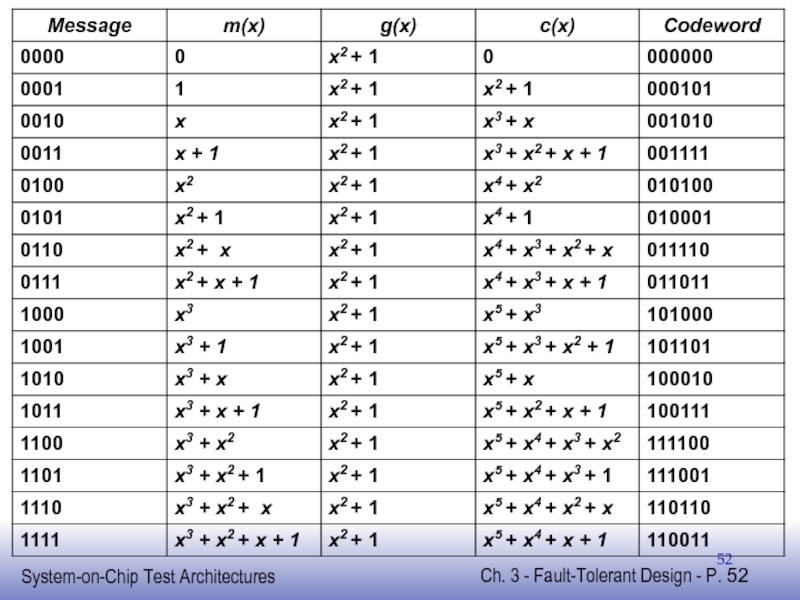
Слайд 53CRC Code
Linear block code
Has G-matrix and H-matrix
G-matrix shifted version of generator

 CRC code generated by g(x)=x2+1")
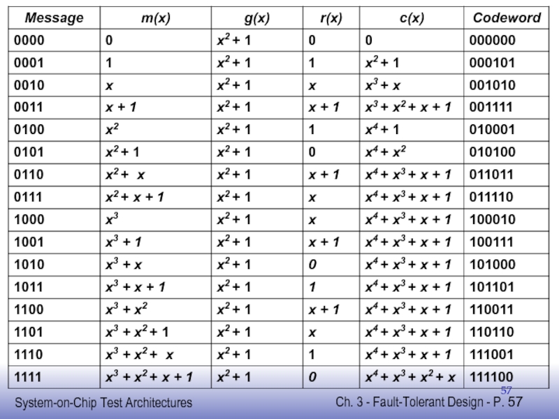
Слайд 55Systematic CRC Codes
To obtain systematic CRC code
codewords formed using Galois division
nice

Слайд 56Galois Division Example
Encode m(x)=x2+x with g(x)=x2+1
Requires dividing m(x)xn-k =x4+x3 by g(x)
Remainder
c(x) = m(x)xn-k+r(x) = (x2+x)(x2)+x+1 = x4+x3+x+1
=x2+x with g(x)=x2+1Requires dividing m(x)xn-k =x4+x3 by g(x)Remainder r(x)=x+1c(x) = m(x)xn-k+r(x) =")
Слайд 58Generating Check Bits for CRC Code
Use LFSR
With characteristic polynomial equal to
Append n-k 0’s to end of message
Example: m(x)=x2+x+1 and g(x)=x3+x+1
Append n-k 0’s to")
Слайд 59Checking CRC Codeword
Checking Received Codeword for Errors
Shift codeword into LFSR
with same
If final state of LFSR non-zero, then error

Слайд 60Selecting Generator Polynomial
Key issue for CRC Codes
If first and last bit
Will detect burst errors of length n-k or less
If generator polynomial is multiple of (x+1)
Will detect any odd number of errors
If g(x) = (x+1)p(x) where p(x) primitive of degree n-k-1 and n < 2n-k-1
Will detect single, double, triple, and odd errors


Слайд 62Fault Tolerance Schemes
Adding Fault Tolerance to Design
Improves dependability of system
Requires redundancy
Hardware
Time
Information

Слайд 63Hardware Redundancy
Involves replicating hardware units
At any level of design
gate-level, module-level, chip-level,
Three Basic Forms
Static (also called Passive)
Masks faults rather than detects them
Dynamic (also called Active)
Detects faults and reconfigures to spare hardware
Hybrid
Combines active and passive approaches

Слайд 64Static Redundancy
Masks faults so no erroneous outputs
Provides uninterrupted operation
Important for real-time
No time to reconfigure or retry operation
Simple self-contained
No need to update or rollback system state

Слайд 65Triple Module Redundancy (TMR)
Well-known static redundancy scheme
Three copies of module
Use majority
Error in one module out-voted by other two
Well-known static redundancy schemeThree copies of moduleUse majority voter to determine final")
Слайд 66TMR Reliability and MTTF
TMR works if any 2 modules work
Rm =
Rv = reliability of voter
MTTF for TMR

Слайд 67Comparison with Simplex
Neglecting fault rate of voter
TMR has lower MTTF, but
Can
Higher reliability for short mission times

Слайд 68Comparison with Simplex
Crossover point
RTMR > Rsimplex when
Mission time shorter than 70%

Слайд 69N-Modular Redundancy (NMR)
NMR
N modules along with majority voter
TMR special case
Number of
As N increases, MTTF decreases
But, reliability for short missions increases
If goal only to tolerate temporary faults
TMR sufficient
NMRN modules along with majority voterTMR special caseNumber of failed modules masked =")
Слайд 70Interwoven Logic
Replace each gate
with 4 gates using inconnection pattern that automatically
Traditionally not as attractive as TMR
Requires lots of area overhead
Renewed interest by researchers investigating emerging nanoelectronic technologies


Слайд 73Dynamic Redundancy
Involves
Detecting fault
Locating faulty hardware unit
Reconfiguring system to use spare fault-free

Слайд 74Unpowered (Cold) Spares
Advantage
Extends lifetime of spares
Equations
Assume spare not failing until powered
Perfect
 SparesAdvantageExtends lifetime of sparesEquationsAssume spare not failing until poweredPerfect reconfiguration capability")
Слайд 75Unpowered (Cold) Spares
One cold spare doubles MTTF
Assuming faults always detected and
Drawback of cold spare
Extra time to power and initialize
Cannot be used to help in detecting faults
Fault detection requires either
periodic offline testing
online testing using time or information redundancy
 SparesOne cold spare doubles MTTFAssuming faults always detected and reconfiguration circuitry never failsDrawback")
Слайд 76Powered (Hot) Spares
Can use spares for online fault detection
One approach is
If outputs mismatch then fault occurred
Run diagnostic procedure to determine which module is faulty and replace with spare
Any number of spares can be used
 SparesCan use spares for online fault detectionOne approach is duplicate-and-compareIf outputs mismatch then")

Слайд 78TMR/Simplex
When one module in TMR fails
Disconnect one of remaining modules
Improves MTTF
TMR/Simplex
Reliability always better than either TMR or Simplex alone


Слайд 80Hybrid Redundancy
Combines both static and dynamic redundancy
Masks faults like static
Detects and

Слайд 81TMR with Spares
If TMR module fails
Replace with spare
can be either hot
While system has three working modules
TMR will provide fault masking for uninterrupted operation

Слайд 82Self-Purging Redundancy
Uses threshold voter instead of majority voter
Threshold voter outputs 1
Otherwise outputs 0
Requires hot spares


Слайд 84Self-Purging Redundancy
Compared with 5MR
Self-purging with 5 modules
Tolerate up to 3 failing
Cannot tolerate two modules simultaneously failing (5MR can)
Compared with TMR with 2 spares
Self-purging with 5 modules
simpler reconfiguration circuitry
requires hot spares (3MR w/spares can use either hot or cold spares)
Cannot tolerate")
Слайд 85Time Redundancy
Advantage
Less hardware
Drawback
Cannot detect permanent faults
If error detected
System needs to rollback

Слайд 86Repeated Execution
Repeat operation twice
Simplest time redundancy approach
Detects temporary faults occurring during
Causes mismatch in results
Can reuse same hardware for both executions
Only one copy of functional hardware needed

Слайд 87Repeated Execution
Requires mechanism for storing and comparing results of both executions
In
Main cost
Additional time for redundant execution and comparison

Слайд 88Multi-threaded Redundant Execution
Can use in processor-based system that can run multiple
Two copies of thread executed concurrently
Results compared when both complete
Take advantage of processor’s built-in capability to exploit processing resources
Reduce execution time
Can significantly reduce performance penalty

Слайд 89Multiple Sampling of Outputs
Done at circuit-level
Sample once at end of normal
Same again after delay of Δt
Two samples compared to detect mismatch
Indicates error occurred
Detect fault whose duration is less than Δt
Performance overhead depends on
Size of Δt relative to normal clock period


Слайд 92Diverse Recomputation
Use same hardware, but perform computation differently second time
Can detect
For arithmetic or logical operations
Shift operands when performing second computation [Patel 1982]
Detects permanent fault affecting only one bit-slice

Слайд 93Information Redundancy
Based on Error Detecting and Correcting Codes
Advantage
Detects both permanent and
Implemented with less hardware overhead than using multiple copies of module
Disadvantage
More complex design

Слайд 94Error Detection
Error detecting codes used to detect errors
If error detected
Rollback to
Retry operation

Слайд 95Rollback
Requires adding storage to save previous state
Amount of rollback depends on
Zero-latency error detection
rollback implemented by preventing system state from updating
If errors detected after n cycles
need rollback restoring system to state at least n clock cycles earlier

Слайд 96Checkpoint
Execution divided into set of operations
Before each operation executed
checkpoint created where
If any error detected during operation
rollback to last checkpoint and retry operation
If multiple retries fail
operation halts and system flags that permanent fault has occurred

Слайд 97Error Detection
Encode outputs of circuit with error detecting code
Non-codeword output indicates

Слайд 98Self-Checking Checker
Has two outputs
Normal error-free case (1,0) or (0,1)
If equal to
Cannot have single error indicator output
Stuck-at 0 fault on output could never be detected
 or (0,1)If equal to each other, then error")
Слайд 99Totally Self-Checking Checker
Requires three properties
Code Disjoint
all codeword inputs mapped to codeword
Fault Secure
for all codeword inputs, checker in presence of fault will either procedure correct codeword output or non-codeword output (not incorrect codeword)
Self-Testing
For each fault, at least one codeword input gives error indication

Слайд 100Duplicate-and-Compare
Equality checker indicates error
Undetected error can occur only if common-mode fault
Only faults after stems detected
Over 100% overhead (including checker)

Слайд 101Single-Bit Parity Code
Totally self-checking checker formed by removing final gate from

Слайд 102Single-Bit Parity Code
Cannot detect even bit errors
Can ensure no even bit
Only single bit errors can occur due to single point fault
Typically requires a lot of overhead

Слайд 103Parity-Check Codes
Each check bit is parity for some set of output
Example: 6 outputs and 3 check bits

Слайд 104Parity-Check Codes
For c check bits and k functional outputs
2ck possible parity
Can choose code based on structure of circuit to minimize undetected error combinations
Fanouts in circuit determine possible error combinations due to single-point fault

Слайд 105Checker for Parity-Check Codes
Constructed from single-bit parity checkers and two-rail checkers


Слайд 107Berger Codes
Inverter-free circuit
Inverters only at primary inputs
Can be synthesized using only
Only unidirectional errors possible for single point faults
Can use unidirectional code
Berger code gives 100% coverage

Слайд 108Constant Weight Codes
Non-separable with lower redundancy
Drawback: need decoding logic to convert
Can use for encoding states of FSM
No need for decoding logic

Слайд 109Error Correction
Information redundancy can also be used to mask errors
Not as
However, very good for memories
Check bits stored with data
Error do not propagate in memories as in logic circuits, so SEC-DED usually sufficient

Слайд 110Error Correction
Memories very dense and prone to errors
Especially due to single-event
SEC-DED check bits stored in memory
32-bit word, SEC-DED requires 7 check bits
Increases size of memory by 7/32=21.9%
64-bit word, SEC-DED requires 8 check bits
Increases size of memory by 8/64=12.5%
 from radiationSEC-DED")

Слайд 112Hamming Code for ECC RAM
Z
1
Z
2
Z
3
Z
4
Z
5
Z
6
Z
7
Z
8
c
1
c
2
c
3
c
4
Parity Group 1
1
1
0
1
1
0
1
0
1
0
0
0
Parity Group 2
1
0
1
1
0
1
1
0
0
1
0
0
Parity Group 3
0
1
1
1
0
0
0
1
0
0
1
0
Parity Group 4
0
0
0
0
1
1
1
1
0
0
0
1

Слайд 113Memory ECC
SEC-DED generally very effective
Memory bit-flips tend to be independent and
If bit-flip occurs, gets corrected next time memory location accessed
Main risk is if memory word not access for long time
Multiple bit-flips could accumulate

Слайд 114Memory Scrubbing
Every location in memory read on periodic basis
Reduces chance of
Can be implemented by having memory controller cycle through memory during idle periods

Слайд 115Multiple-Bit Upsets (MBU)
Can occur due to single SEU
Typically occur in adjacent
Memory interleaving used
To prevent MBUs from resulting in multiple bit errors in same word
Can occur due to single SEUTypically occur in adjacent memory cellsMemory interleaving usedTo")
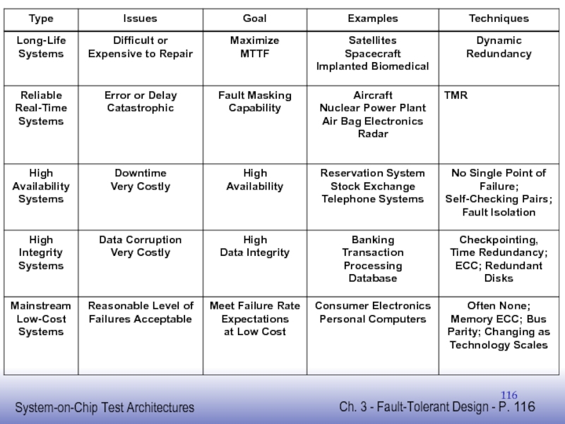
Слайд 117Concluding Remarks
Many different fault-tolerant schemes
Choosing scheme depends on
Types of faults to
Temporary or permanent
Single or multiple point failures
etc.
Design constraints
Area, performance, power, etc.

Слайд 118Concluding Remarks
As technology scales
Circuits increasingly prone to failure
Achieving sufficient fault tolerance