- Главная
- Разное
- Дизайн
- Бизнес и предпринимательство
- Аналитика
- Образование
- Развлечения
- Красота и здоровье
- Финансы
- Государство
- Путешествия
- Спорт
- Недвижимость
- Армия
- Графика
- Культурология
- Еда и кулинария
- Лингвистика
- Английский язык
- Астрономия
- Алгебра
- Биология
- География
- Детские презентации
- Информатика
- История
- Литература
- Маркетинг
- Математика
- Медицина
- Менеджмент
- Музыка
- МХК
- Немецкий язык
- ОБЖ
- Обществознание
- Окружающий мир
- Педагогика
- Русский язык
- Технология
- Физика
- Философия
- Химия
- Шаблоны, картинки для презентаций
- Экология
- Экономика
- Юриспруденция
Deep belief nets презентация
Содержание
- 1. Deep belief nets
- 2. Some things you will learn in this
- 3. A spectrum of machine learning tasks Low-dimensional
- 4. Historical background: First generation neural networks Perceptrons
- 5. Second generation neural networks (~1985) input vector
- 6. A temporary digression Vapnik and his co-workers
- 7. What is wrong with back-propagation? It requires
- 8. Overcoming the limitations of back-propagation Keep
- 9. Belief Nets A belief net is
- 10. Stochastic binary units (Bernoulli variables) These have
- 11. Learning Deep Belief Nets It is
- 12. The learning rule for sigmoid belief nets
- 13. Explaining away (Judea Pearl) Even if two
- 14. Why it is usually very hard to
- 15. Two types of generative neural network If
- 16. Restricted Boltzmann Machines (Smolensky ,1986, called them
- 17. The Energy of a joint configuration (ignoring
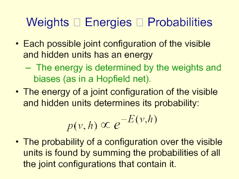
- 18. Weights ? Energies ? Probabilities Each
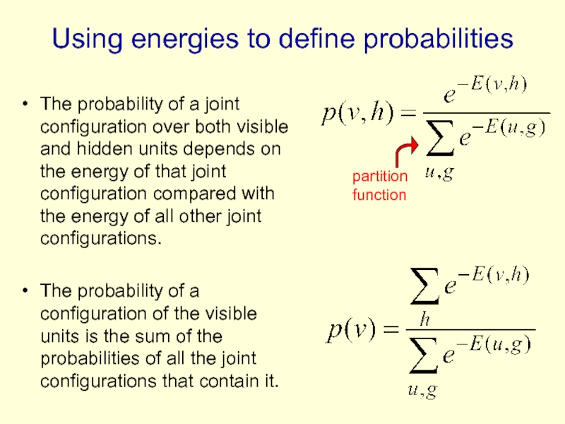
- 19. Using energies to define probabilities The probability
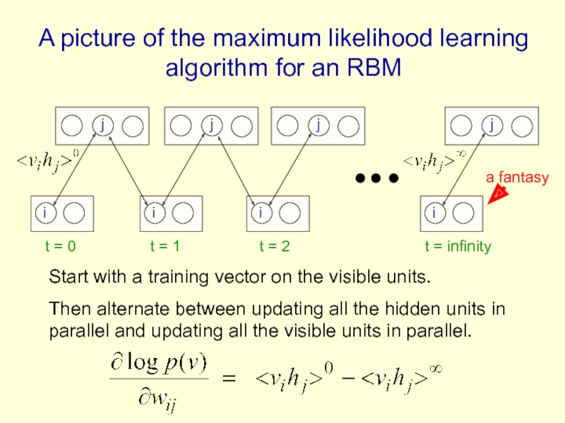
- 20. A picture of the maximum
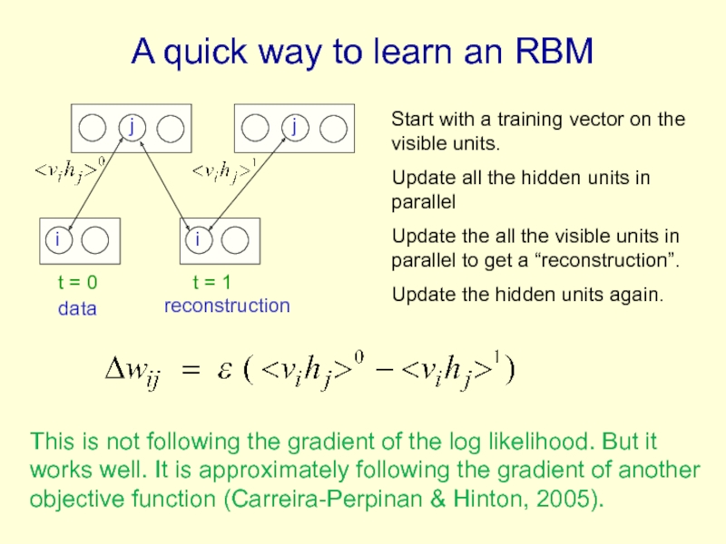
- 21. A quick way to learn an
- 22. How to learn a set of features
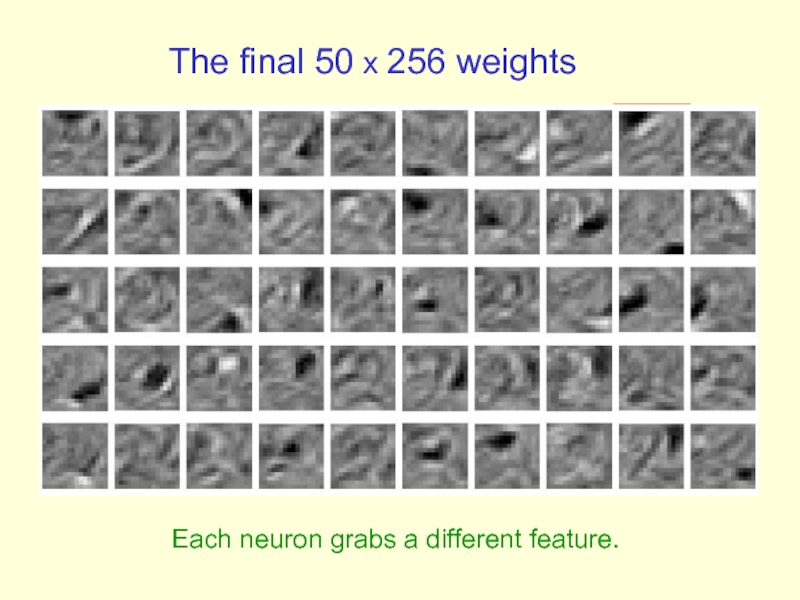
- 23. The final 50 x 256 weights Each neuron grabs a different feature.
- 24. Reconstruction from activated binary features Data
- 25. Three ways to combine probability density models
- 26. Training a deep network (the main reason
- 27. The generative model after learning 3 layers
- 28. Why does greedy learning work?
- 29. Why does greedy learning work? Each
- 30. Why does greedy learning work? The weights,
- 31. Which distributions are factorial in a directed
- 32. Why does greedy learning fail in
- 33. A model of digit recognition 2000 top-level
- 34. Fine-tuning with a contrastive version of the
- 35. Show the movie of the network generating
- 36. Samples generated by letting the associative memory
- 37. Examples of correctly recognized handwritten digits that
- 38. How well does it discriminate on MNIST
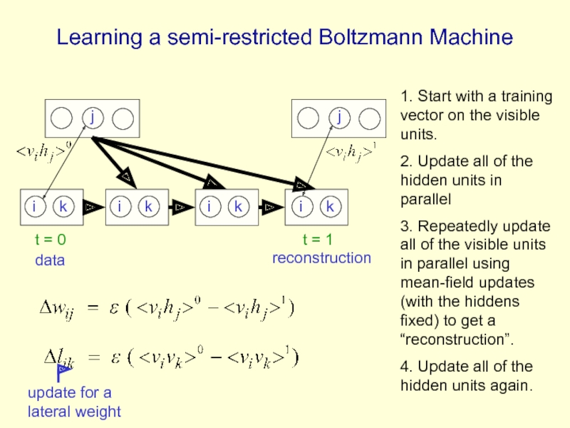
- 39. Unsupervised “pre-training” also helps for models that
- 40. Another view of why layer-by-layer learning
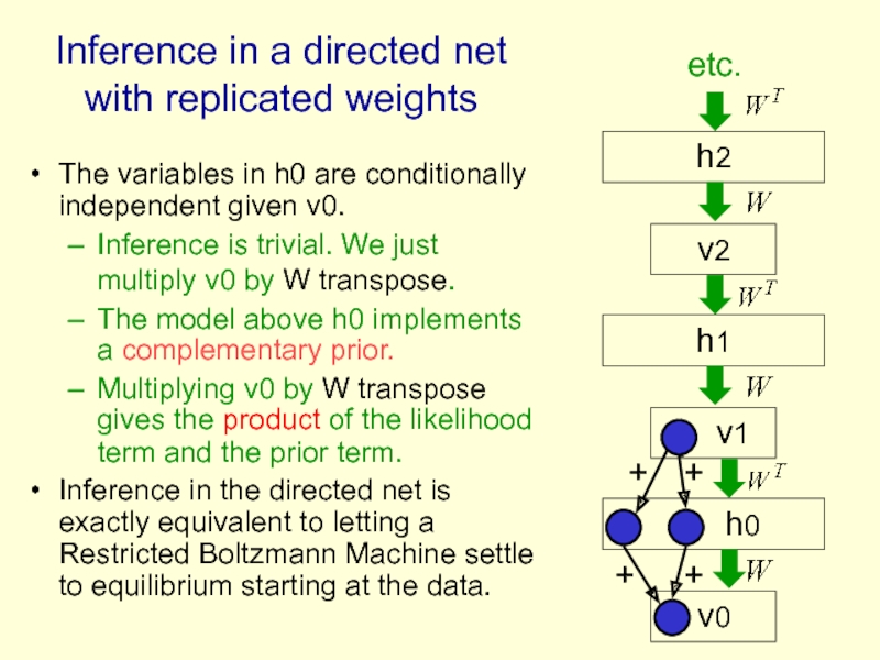
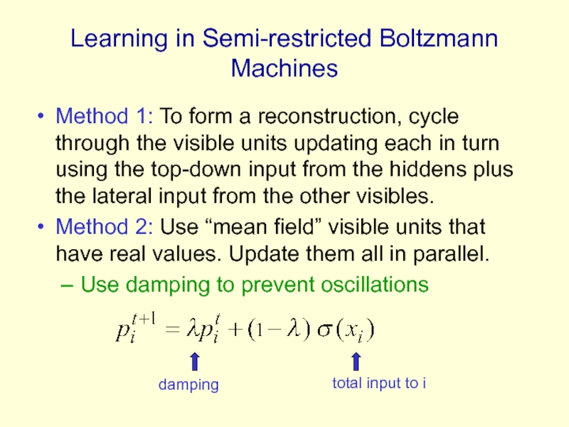
- 41. An infinite sigmoid belief net that is
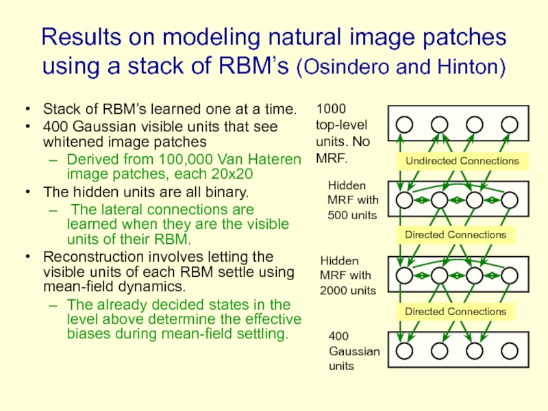
- 42. The variables in h0 are conditionally independent
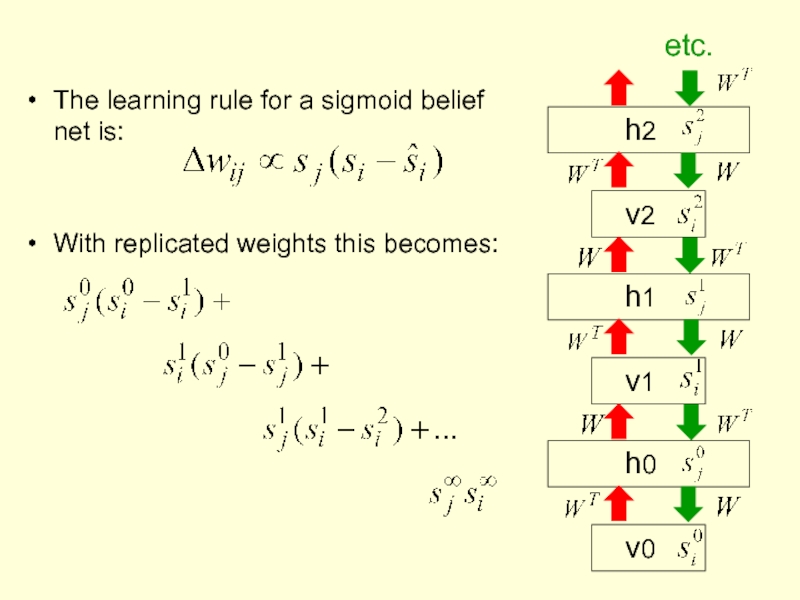
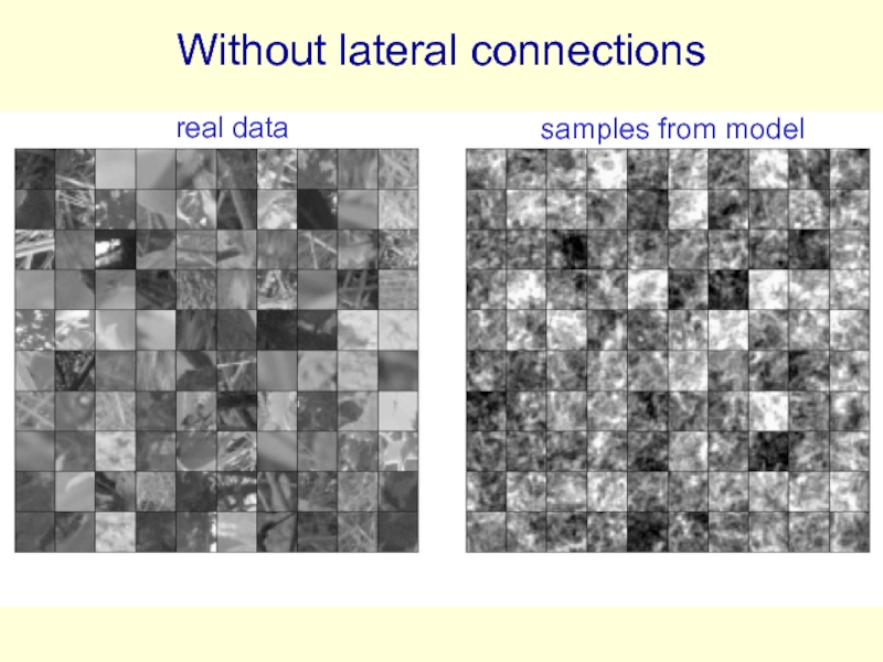
- 43. The learning rule for a sigmoid belief
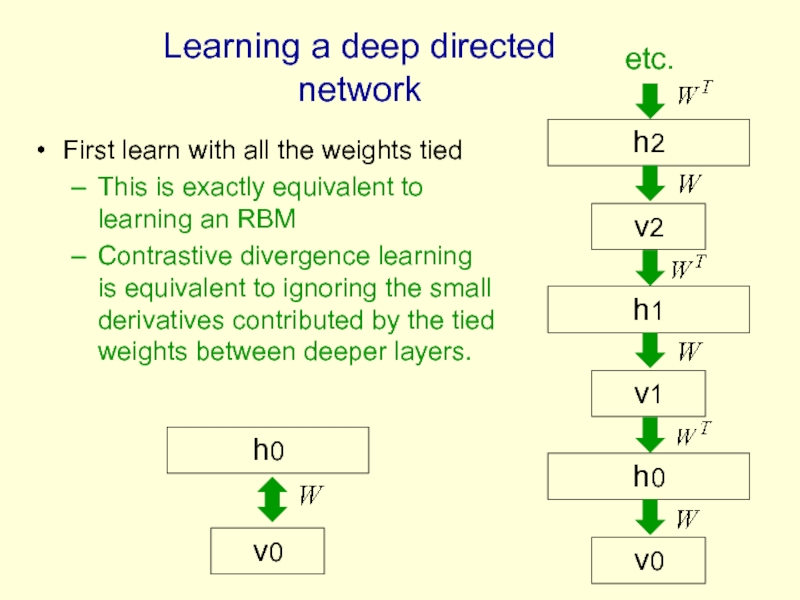
- 44. First learn with all the weights tied
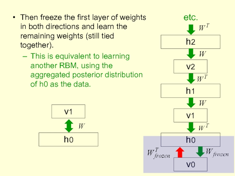
- 45. Then freeze the first layer of weights
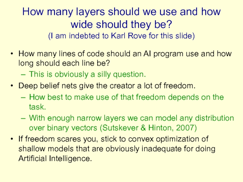
- 46. How many layers should we use and
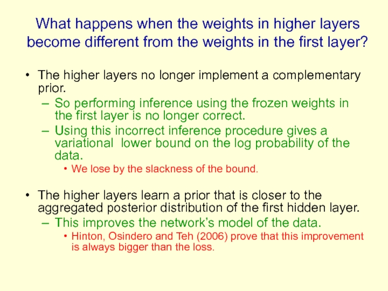
- 47. What happens when the weights in higher
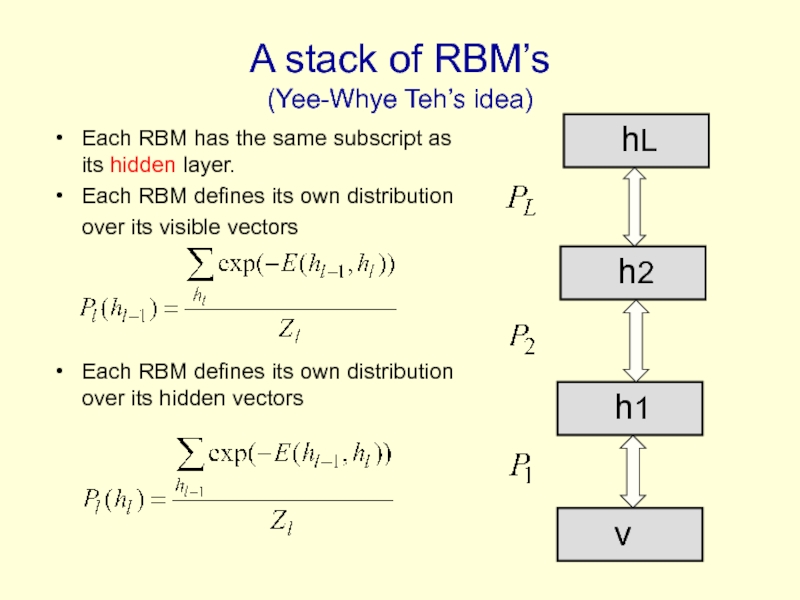
- 48. A stack of RBM’s (Yee-Whye Teh’s idea)
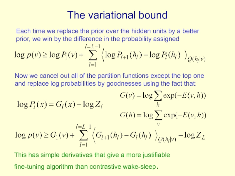
- 49. The variational bound Now we cancel out
- 50. Summary so far Restricted Boltzmann Machines provide
- 51. Overview of the rest of the tutorial
- 52. BREAK
- 53. Fine-tuning for discrimination First learn one layer
- 54. Why backpropagation works better after greedy pre-training
- 55. First, model the distribution of digit images
- 56. Results on permutation-invariant MNIST task Very carefully
- 57. Combining deep belief nets with Gaussian processes
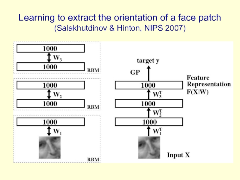
- 58. Learning to extract the orientation of a face patch (Salakhutdinov & Hinton, NIPS 2007)
- 59. The training and test sets 11,000 unlabeled
- 60. The root mean squared error in the
- 61. Modeling real-valued data For images of digits
- 62. The free-energy of a mean-field logistic unit
- 63. An RBM with real-valued visible units
- 64. Deep Autoencoders (Hinton & Salakhutdinov, 2006) They
- 65. A comparison of methods for compressing digit
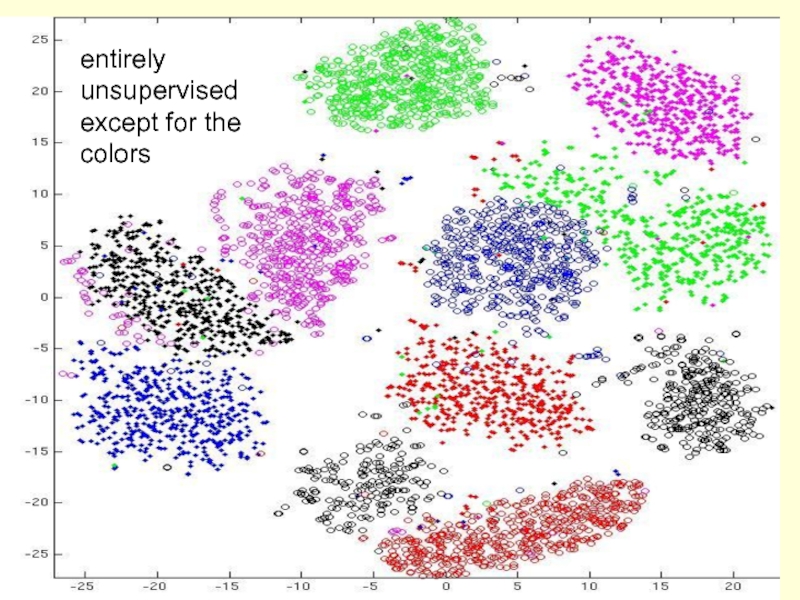
- 66. Do the 30-D codes found by the
- 67. entirely unsupervised except for the colors
- 68. Retrieving documents that are similar to a
- 69. How to compress the count vector
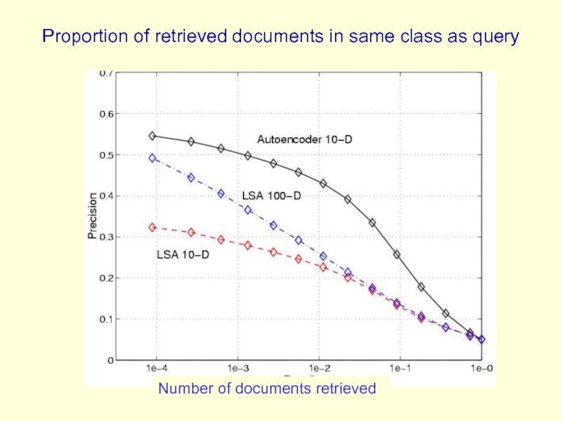
- 70. Performance of the autoencoder at document retrieval
- 71. Proportion of retrieved documents in same class as query Number of documents retrieved
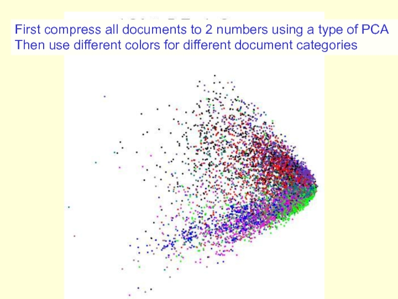
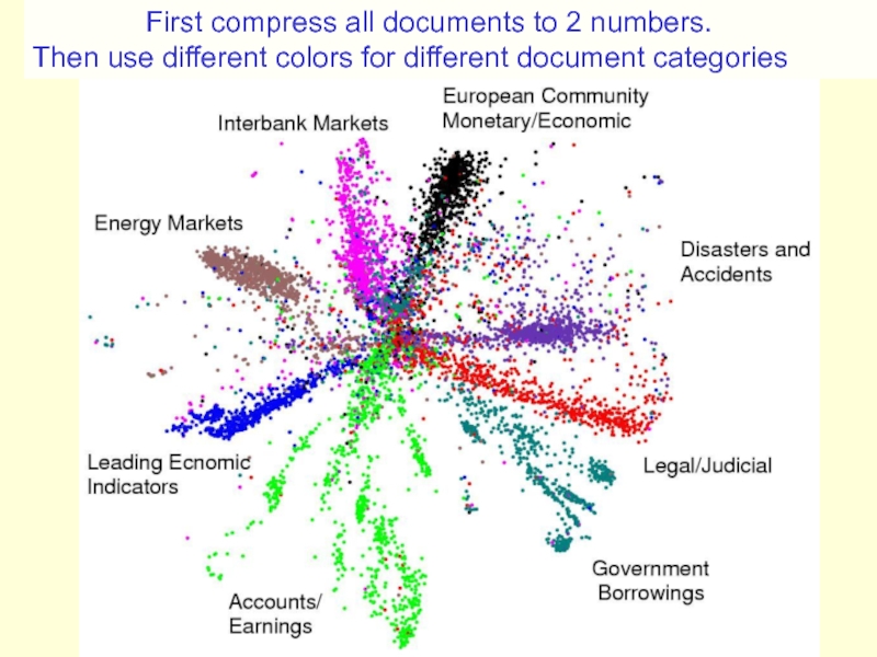
- 72. First compress all documents to 2
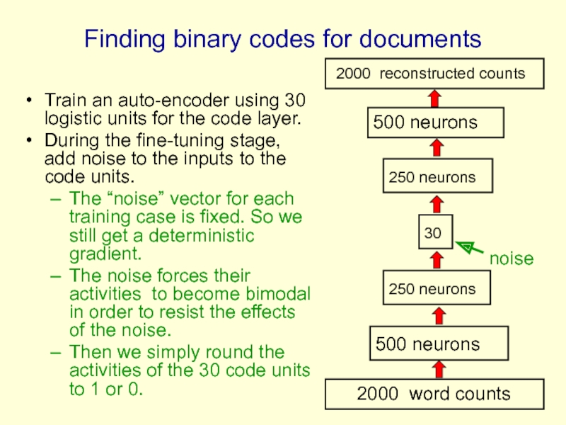
- 74. Finding binary codes for documents Train
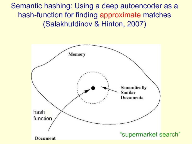
- 75. Semantic hashing: Using a deep autoencoder as
- 76. How good is a shortlist found this
- 77. Time series models Inference is difficult in
- 78. Time series models If we really need
- 79. The conditional RBM model (Sutskever &
- 80. Why the autoregressive connections do not cause
- 81. Generating from a learned model The inputs
- 82. Stacking temporal RBM’s Treat the hidden activities
- 83. An application to modeling motion capture
- 84. Modeling multiple types of motion We can
- 85. Show Graham Taylor’s movies available at www.cs.toronto/~hinton
- 86. Generating the parts of an object
- 87. Semi-restricted Boltzmann Machines We restrict the connectivity
- 88. Learning a semi-restricted Boltzmann Machine
- 89. Learning in Semi-restricted Boltzmann Machines Method
- 90. Results on modeling natural image patches using
- 91. Without lateral connections real data samples from model
- 92. With lateral connections real data samples from model
- 93. A funny way to use an MRF
- 94. Why do we whiten data? Images typically
- 95. Whitening the learning signal instead of the
- 96. Towards a more powerful, multi-linear stackable learning
- 97. Higher order Boltzmann machines (Sejnowski, ~1986) The
- 98. A picture of a conditional, higher-order
- 99. Using conditional higher-order Boltzmann machines to model
- 100. Readings on deep belief nets A reading
Слайд 12007 NIPS Tutorial on:
Deep Belief Nets
Geoffrey Hinton
Canadian Institute for Advanced
&
Department of Computer Science
University of Toronto
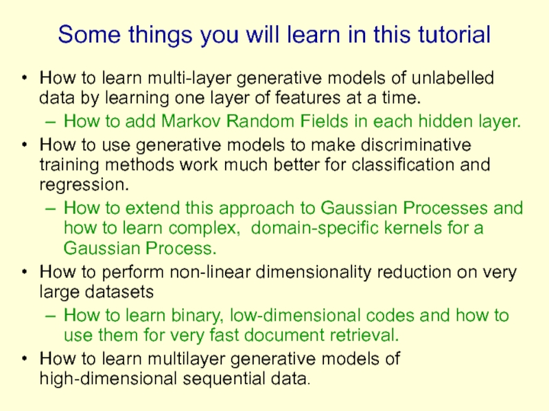
Слайд 2Some things you will learn in this tutorial
How to learn multi-layer
How to add Markov Random Fields in each hidden layer.
How to use generative models to make discriminative training methods work much better for classification and regression.
How to extend this approach to Gaussian Processes and how to learn complex, domain-specific kernels for a Gaussian Process.
How to perform non-linear dimensionality reduction on very large datasets
How to learn binary, low-dimensional codes and how to use them for very fast document retrieval.
How to learn multilayer generative models of high-dimensional sequential data.
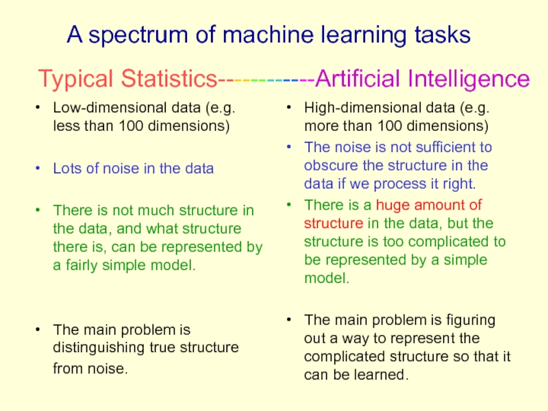
Слайд 3A spectrum of machine learning tasks
Low-dimensional data (e.g. less than 100
Lots of noise in the data
There is not much structure in the data, and what structure there is, can be represented by a fairly simple model.
The main problem is distinguishing true structure from noise.
High-dimensional data (e.g. more than 100 dimensions)
The noise is not sufficient to obscure the structure in the data if we process it right.
There is a huge amount of structure in the data, but the structure is too complicated to be represented by a simple model.
The main problem is figuring out a way to represent the complicated structure so that it can be learned.
Typical Statistics------------Artificial Intelligence
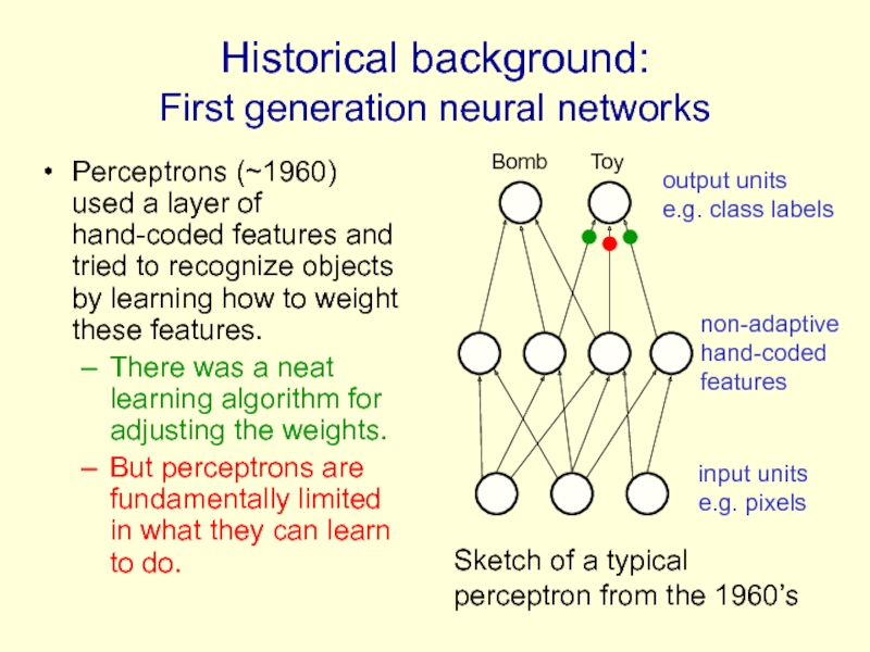
Слайд 4Historical background:
First generation neural networks
Perceptrons (~1960) used a layer of hand-coded
There was a neat learning algorithm for adjusting the weights.
But perceptrons are fundamentally limited in what they can learn to do.
non-adaptive
hand-coded
features
output units e.g. class labels
input units e.g. pixels
Sketch of a typical perceptron from the 1960’s
Bomb
Toy
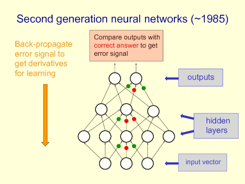
Слайд 5Second generation neural networks (~1985)
input vector
hidden layers
outputs
Back-propagate
Compare outputs with correct answer to get error signal
Слайд 6A temporary digression
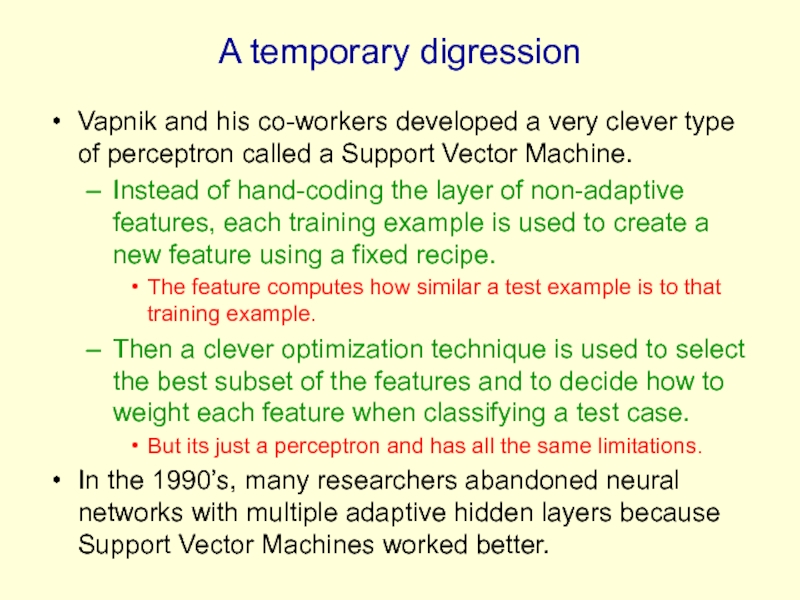
Vapnik and his co-workers developed a very clever type
Instead of hand-coding the layer of non-adaptive features, each training example is used to create a new feature using a fixed recipe.
The feature computes how similar a test example is to that training example.
Then a clever optimization technique is used to select the best subset of the features and to decide how to weight each feature when classifying a test case.
But its just a perceptron and has all the same limitations.
In the 1990’s, many researchers abandoned neural networks with multiple adaptive hidden layers because Support Vector Machines worked better.
Слайд 7What is wrong with back-propagation?
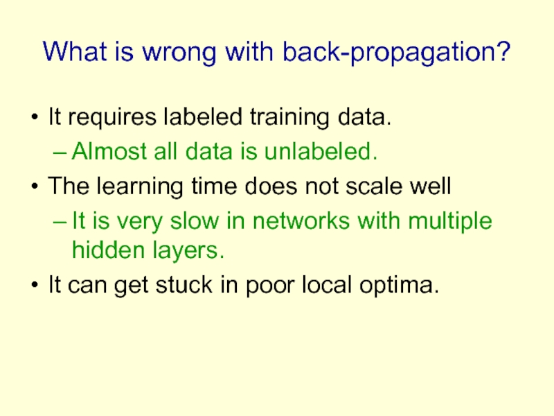
It requires labeled training data.
Almost all data
The learning time does not scale well
It is very slow in networks with multiple hidden layers.
It can get stuck in poor local optima.
Слайд 8Overcoming the limitations of back-propagation
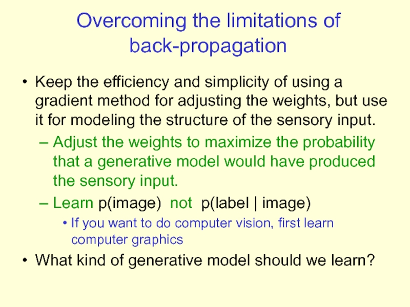
Keep the efficiency and simplicity of using
Adjust the weights to maximize the probability that a generative model would have produced the sensory input.
Learn p(image) not p(label | image)
If you want to do computer vision, first learn computer graphics
What kind of generative model should we learn?
Слайд 9 Belief Nets
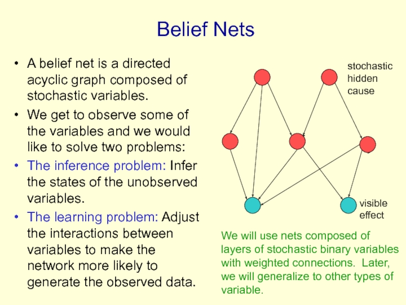
A belief net is a directed acyclic graph composed
We get to observe some of the variables and we would like to solve two problems:
The inference problem: Infer the states of the unobserved variables.
The learning problem: Adjust the interactions between variables to make the network more likely to generate the observed data.
stochastic
hidden cause
visible
effect
We will use nets composed of layers of stochastic binary variables with weighted connections. Later, we will generalize to other types of variable.
Слайд 10Stochastic binary units
(Bernoulli variables)
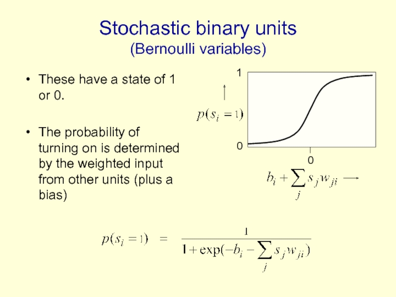
These have a state of 1 or 0.
The
0
0
1
Слайд 11 Learning Deep Belief Nets
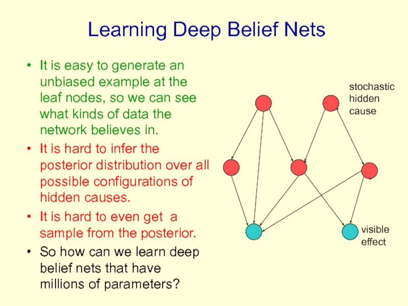
It is easy to generate an unbiased
It is hard to infer the posterior distribution over all possible configurations of hidden causes.
It is hard to even get a sample from the posterior.
So how can we learn deep belief nets that have millions of parameters?
stochastic
hidden cause
visible
effect
Слайд 12The learning rule for sigmoid belief nets
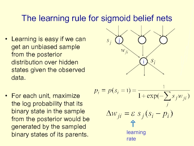
Learning is easy if we
For each unit, maximize the log probability that its binary state in the sample from the posterior would be generated by the sampled binary states of its parents.
j
i
learning rate
Слайд 13Explaining away (Judea Pearl)
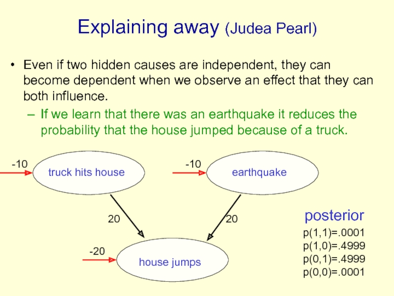
Even if two hidden causes are independent, they
If we learn that there was an earthquake it reduces the probability that the house jumped because of a truck.
truck hits house
earthquake
house jumps
20
20
-20
-10
-10
p(1,1)=.0001
p(1,0)=.4999
p(0,1)=.4999
p(0,0)=.0001
posterior
Слайд 14Why it is usually very hard to learn sigmoid
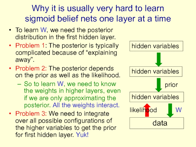
To learn W, we need the posterior distribution in the first hidden layer.
Problem 1: The posterior is typically complicated because of “explaining away”.
Problem 2: The posterior depends on the prior as well as the likelihood.
So to learn W, we need to know the weights in higher layers, even if we are only approximating the posterior. All the weights interact.
Problem 3: We need to integrate over all possible configurations of the higher variables to get the prior for first hidden layer. Yuk!
data
hidden variables
hidden variables
hidden variables
likelihood
W
prior
Слайд 15Two types of generative neural network
If we connect binary stochastic neurons
If we connect binary stochastic neurons using symmetric connections we get a Boltzmann Machine (Hinton & Sejnowski, 1983).
If we restrict the connectivity in a special way, it is easy to learn a Boltzmann machine.
Слайд 16Restricted Boltzmann Machines
(Smolensky ,1986, called them “harmoniums”)
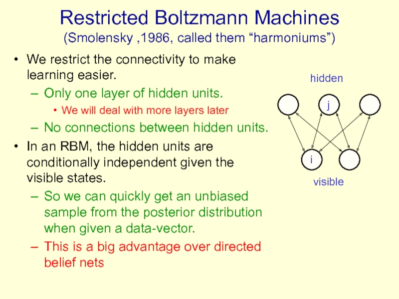
We restrict the connectivity to
Only one layer of hidden units.
We will deal with more layers later
No connections between hidden units.
In an RBM, the hidden units are conditionally independent given the visible states.
So we can quickly get an unbiased sample from the posterior distribution when given a data-vector.
This is a big advantage over directed belief nets
hidden
i
j
visible
Слайд 17The Energy of a joint configuration
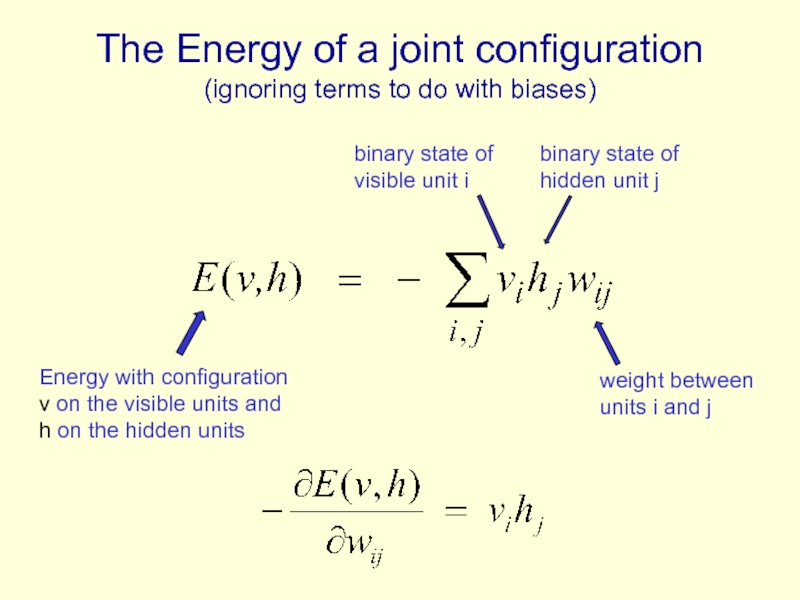
(ignoring terms to do with biases)
weight
Energy with configuration v on the visible units and h on the hidden units
binary state of visible unit i
binary state of hidden unit j
Слайд 18Weights ? Energies ? Probabilities
Each possible joint configuration of the visible
The energy is determined by the weights and biases (as in a Hopfield net).
The energy of a joint configuration of the visible and hidden units determines its probability:
The probability of a configuration over the visible units is found by summing the probabilities of all the joint configurations that contain it.
Слайд 19Using energies to define probabilities
The probability of a joint configuration over
The probability of a configuration of the visible units is the sum of the probabilities of all the joint configurations that contain it.
partition function
Слайд 20
A picture of the maximum likelihood learning algorithm for an RBM
i
j
i
j
i
j
i
j
t
Start with a training vector on the visible units.
Then alternate between updating all the hidden units in parallel and updating all the visible units in parallel.
a fantasy
Слайд 21
A quick way to learn an RBM
i
j
i
j
t = 0
Start with a training vector on the visible units.
Update all the hidden units in parallel
Update the all the visible units in parallel to get a “reconstruction”.
Update the hidden units again.
This is not following the gradient of the log likelihood. But it works well. It is approximately following the gradient of another objective function (Carreira-Perpinan & Hinton, 2005).
reconstruction
data
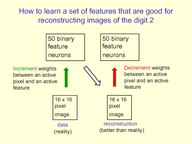
Слайд 22How to learn a set of features that are good for
50 binary feature neurons
16 x 16 pixel image
50 binary feature neurons
16 x 16 pixel image
Increment weights between an active pixel and an active feature
Decrement weights between an active pixel and an active feature
data (reality)
reconstruction (better than reality)
Слайд 24
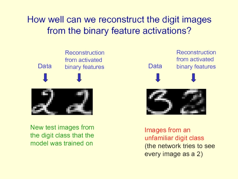
Reconstruction from activated binary features
Data
Reconstruction from activated binary features
Data
How well can
New test images from the digit class that the model was trained on
Images from an unfamiliar digit class (the network tries to see every image as a 2)
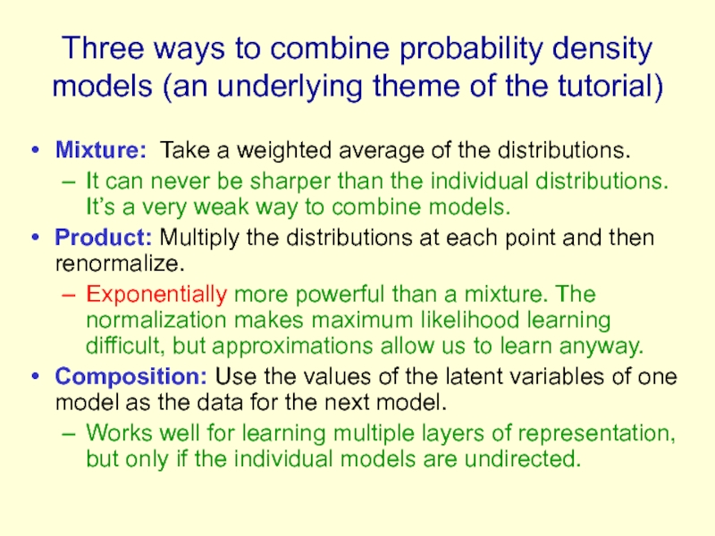
Слайд 25Three ways to combine probability density models (an underlying theme of
Mixture: Take a weighted average of the distributions.
It can never be sharper than the individual distributions. It’s a very weak way to combine models.
Product: Multiply the distributions at each point and then renormalize.
Exponentially more powerful than a mixture. The normalization makes maximum likelihood learning difficult, but approximations allow us to learn anyway.
Composition: Use the values of the latent variables of one model as the data for the next model.
Works well for learning multiple layers of representation, but only if the individual models are undirected.
Слайд 26Training a deep network
(the main reason RBM’s are interesting)
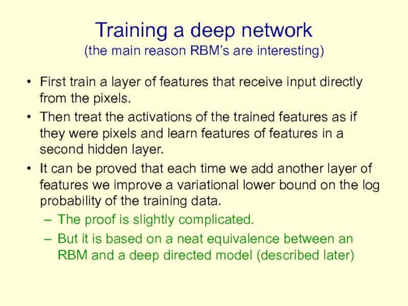
First train a
Then treat the activations of the trained features as if they were pixels and learn features of features in a second hidden layer.
It can be proved that each time we add another layer of features we improve a variational lower bound on the log probability of the training data.
The proof is slightly complicated.
But it is based on a neat equivalence between an RBM and a deep directed model (described later)
Слайд 27The generative model after learning 3 layers
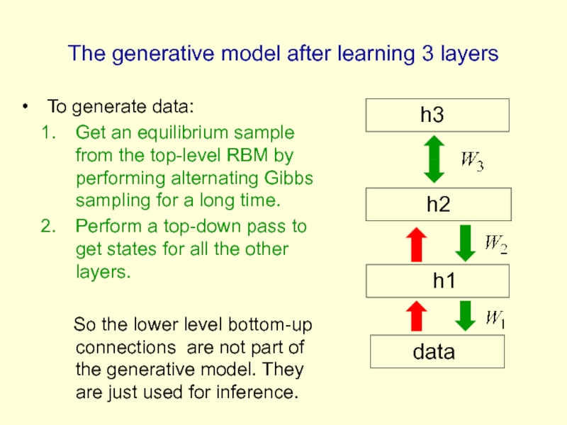
To generate data:
Get an
Perform a top-down pass to get states for all the other layers.
So the lower level bottom-up connections are not part of the generative model. They are just used for inference.
h2
data
h1
h3
Слайд 28Why does greedy learning work? An aside: Averaging
If you average some factorial distributions, you do NOT get a factorial distribution.
In an RBM, the posterior over the hidden units is factorial for each visible vector.
But the aggregated posterior over all training cases is not factorial (even if the data was generated by the RBM itself).
Слайд 29
Why does greedy learning work?
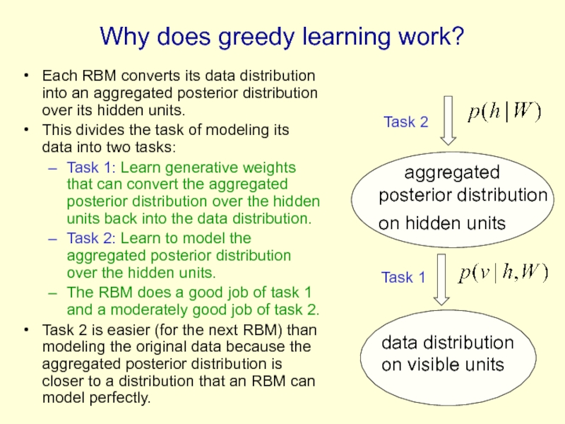
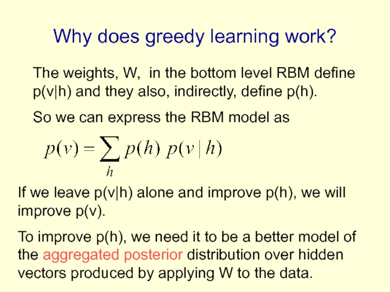
Each RBM converts its data distribution into
This divides the task of modeling its data into two tasks:
Task 1: Learn generative weights that can convert the aggregated posterior distribution over the hidden units back into the data distribution.
Task 2: Learn to model the aggregated posterior distribution over the hidden units.
The RBM does a good job of task 1 and a moderately good job of task 2.
Task 2 is easier (for the next RBM) than modeling the original data because the aggregated posterior distribution is closer to a distribution that an RBM can model perfectly.
data distribution on visible units
aggregated posterior distribution on hidden units
Task 2
Task 1
Слайд 30Why does greedy learning work?
The weights, W, in the bottom level
So we can express the RBM model as
If we leave p(v|h) alone and improve p(h), we will improve p(v).
To improve p(h), we need it to be a better model of the aggregated posterior distribution over hidden vectors produced by applying W to the data.
Слайд 31Which distributions are factorial in a directed belief net?
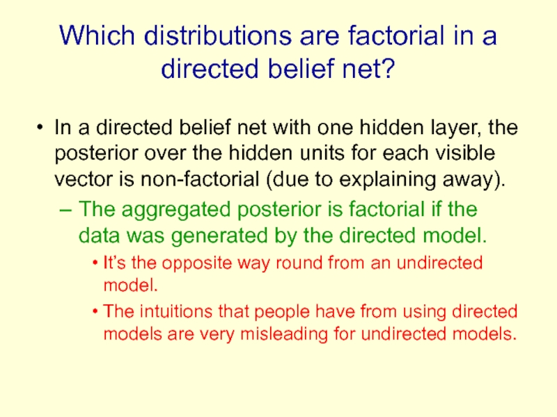
In a directed
The aggregated posterior is factorial if the data was generated by the directed model.
It’s the opposite way round from an undirected model.
The intuitions that people have from using directed models are very misleading for undirected models.
Слайд 32
Why does greedy learning fail in a directed module?
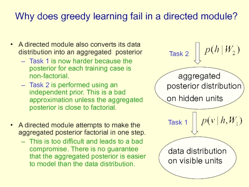
A directed module
Task 1 is now harder because the posterior for each training case is non-factorial.
Task 2 is performed using an independent prior. This is a bad approximation unless the aggregated posterior is close to factorial.
A directed module attempts to make the aggregated posterior factorial in one step.
This is too difficult and leads to a bad compromise. There is no guarantee that the aggregated posterior is easier to model than the data distribution.
data distribution on visible units
Task 2
Task 1
aggregated posterior distribution on hidden units
Слайд 33A model of digit recognition
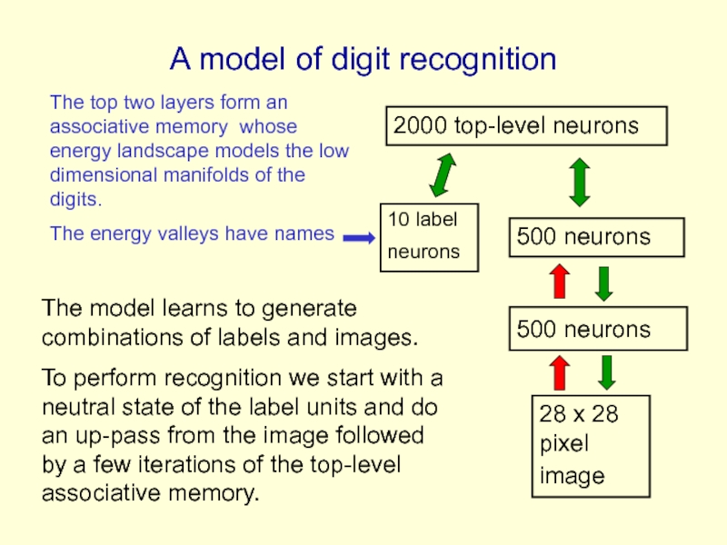
2000 top-level neurons
500 neurons
500 neurons
28 x
10 label neurons
The model learns to generate combinations of labels and images.
To perform recognition we start with a neutral state of the label units and do an up-pass from the image followed by a few iterations of the top-level associative memory.
The top two layers form an associative memory whose energy landscape models the low dimensional manifolds of the digits.
The energy valleys have names
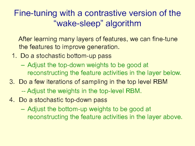
Слайд 34Fine-tuning with a contrastive version of the “wake-sleep” algorithm
After
1. Do a stochastic bottom-up pass
Adjust the top-down weights to be good at reconstructing the feature activities in the layer below.
Do a few iterations of sampling in the top level RBM
-- Adjust the weights in the top-level RBM.
Do a stochastic top-down pass
Adjust the bottom-up weights to be good at reconstructing the feature activities in the layer above.
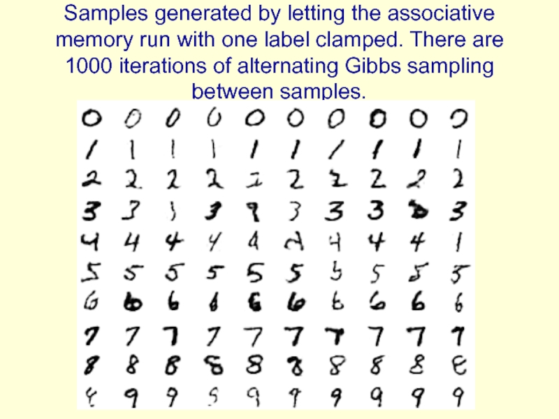
Слайд 36Samples generated by letting the associative memory run with one label
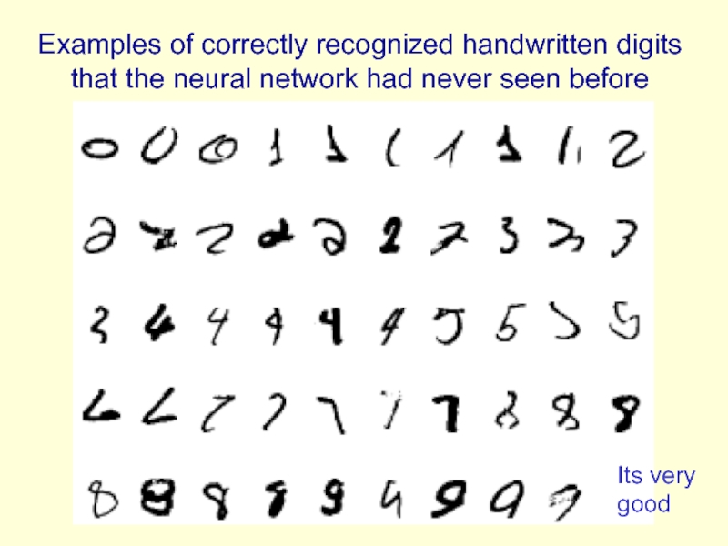
Слайд 37Examples of correctly recognized handwritten digits that the neural network had never
Its very good
Слайд 38How well does it discriminate on MNIST test set with no
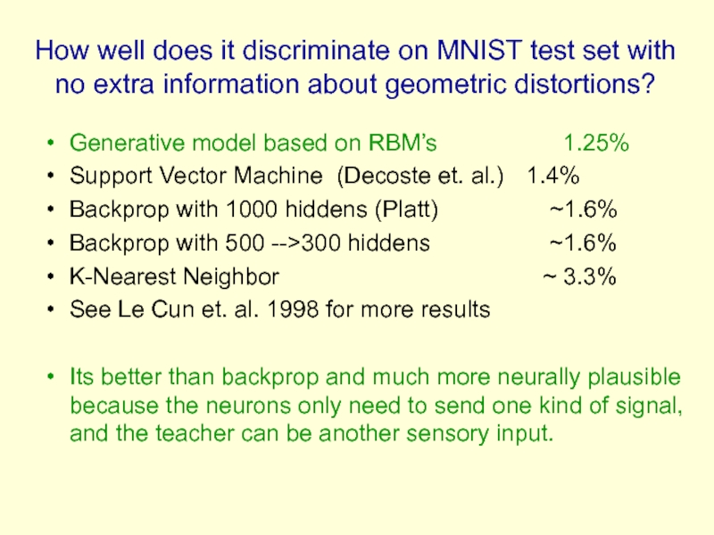
Generative model based on RBM’s 1.25%
Support Vector Machine (Decoste et. al.) 1.4%
Backprop with 1000 hiddens (Platt) ~1.6%
Backprop with 500 -->300 hiddens ~1.6%
K-Nearest Neighbor ~ 3.3%
See Le Cun et. al. 1998 for more results
Its better than backprop and much more neurally plausible because the neurons only need to send one kind of signal, and the teacher can be another sensory input.
Слайд 39Unsupervised “pre-training” also helps for models that have more data and
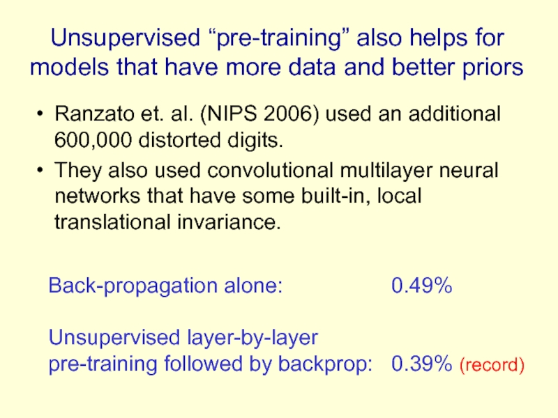
Ranzato et. al. (NIPS 2006) used an additional 600,000 distorted digits.
They also used convolutional multilayer neural networks that have some built-in, local translational invariance.
Back-propagation alone: 0.49%
Unsupervised layer-by-layer
pre-training followed by backprop: 0.39% (record)
Слайд 40Another view of why layer-by-layer learning works
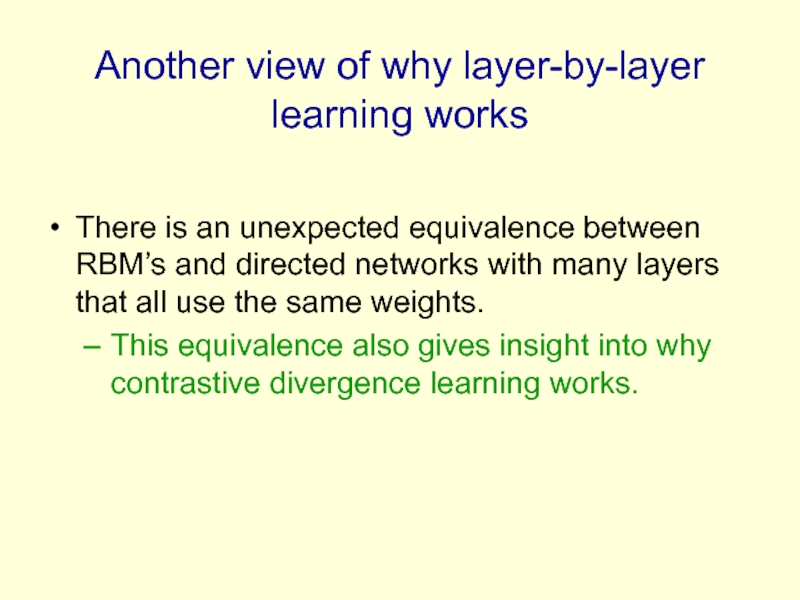
There is an unexpected
This equivalence also gives insight into why contrastive divergence learning works.
Слайд 41An infinite sigmoid belief net that is equivalent to an RBM
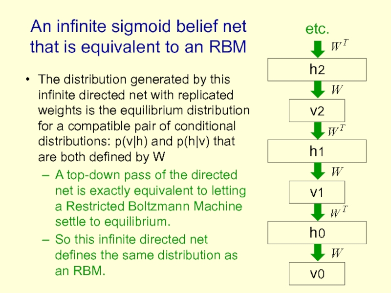
The
A top-down pass of the directed net is exactly equivalent to letting a Restricted Boltzmann Machine settle to equilibrium.
So this infinite directed net defines the same distribution as an RBM.
v1
h1
v0
h0
v2
h2
etc.
Слайд 42The variables in h0 are conditionally independent given v0.
Inference is trivial.
The model above h0 implements a complementary prior.
Multiplying v0 by W transpose gives the product of the likelihood term and the prior term.
Inference in the directed net is exactly equivalent to letting a Restricted Boltzmann Machine settle to equilibrium starting at the data.
Inference in a directed net with replicated weights
v1
h1
v0
h0
v2
h2
etc.
+
+
+
+
Слайд 43The learning rule for a sigmoid belief net is:
With replicated weights
v1
h1
v0
h0
v2
h2
etc.
Слайд 44First learn with all the weights tied
This is exactly equivalent to
Contrastive divergence learning is equivalent to ignoring the small derivatives contributed by the tied weights between deeper layers.
Learning a deep directed network
v1
h1
v0
h0
v2
h2
etc.
v0
h0
Слайд 45Then freeze the first layer of weights in both directions and
This is equivalent to learning another RBM, using the aggregated posterior distribution of h0 as the data.
v1
h1
v0
h0
v2
h2
etc.
v1
h0
Слайд 46How many layers should we use and how wide should they
How many lines of code should an AI program use and how long should each line be?
This is obviously a silly question.
Deep belief nets give the creator a lot of freedom.
How best to make use of that freedom depends on the task.
With enough narrow layers we can model any distribution over binary vectors (Sutskever & Hinton, 2007)
If freedom scares you, stick to convex optimization of shallow models that are obviously inadequate for doing Artificial Intelligence.
Слайд 47What happens when the weights in higher layers become different from
The higher layers no longer implement a complementary prior.
So performing inference using the frozen weights in the first layer is no longer correct.
Using this incorrect inference procedure gives a variational lower bound on the log probability of the data.
We lose by the slackness of the bound.
The higher layers learn a prior that is closer to the aggregated posterior distribution of the first hidden layer.
This improves the network’s model of the data.
Hinton, Osindero and Teh (2006) prove that this improvement is always bigger than the loss.
Слайд 48A stack of RBM’s
(Yee-Whye Teh’s idea)
Each RBM has the same subscript
Each RBM defines its own distribution over its visible vectors
Each RBM defines its own distribution over its hidden vectors
v
h1
h2
hL
Слайд 49The variational bound
Now we cancel out all of the partition functions
This has simple derivatives that give a more justifiable fine-tuning algorithm than contrastive wake-sleep.
Each time we replace the prior over the hidden units by a better prior, we win by the difference in the probability assigned
Слайд 50Summary so far
Restricted Boltzmann Machines provide a simple way to learn
Maximum likelihood learning is computationally expensive because of the normalization term, but contrastive divergence learning is fast and usually works well.
Many layers of representation can be learned by treating the hidden states of one RBM as the visible data for training the next RBM (a composition of experts).
This creates good generative models that can then be fine-tuned.
Contrastive wake-sleep can fine-tune generation.
Слайд 51Overview of the rest of the tutorial
How to fine-tune a greedily
How to learn a kernel for a Gaussian process.
How to use deep belief nets for non-linear dimensionality reduction and document retrieval.
How to use deep belief nets for sequential data.
How to learn a generative hierarchy of conditional random fields.
Слайд 53Fine-tuning for discrimination
First learn one layer at a time greedily.
Then treat
Contrastive wake-sleep is one way of fine-tuning the model to be better at generation.
Backpropagation can be used to fine-tune the model for better discrimination.
This overcomes many of the limitations of standard backpropagation.
Слайд 54Why backpropagation works better after greedy pre-training
Greedily learning one layer at
We do not start backpropagation until we already have sensible weights that already do well at the task.
So the initial gradients are sensible and backprop only needs to perform a local search.
Most of the information in the final weights comes from modeling the distribution of input vectors.
The precious information in the labels is only used for the final fine-tuning. It slightly modifies the features. It does not need to discover features.
This type of backpropagation works well even if most of the training data is unlabeled. The unlabeled data is still very useful for discovering good features.
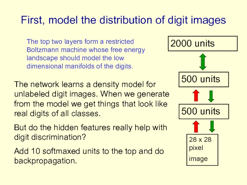
Слайд 55First, model the distribution of digit images
2000 units
500 units
500 units
28 x 28 pixel image
The network learns a density model for unlabeled digit images. When we generate from the model we get things that look like real digits of all classes.
But do the hidden features really help with digit discrimination?
Add 10 softmaxed units to the top and do backpropagation.
The top two layers form a restricted Boltzmann machine whose free energy landscape should model the low dimensional manifolds of the digits.
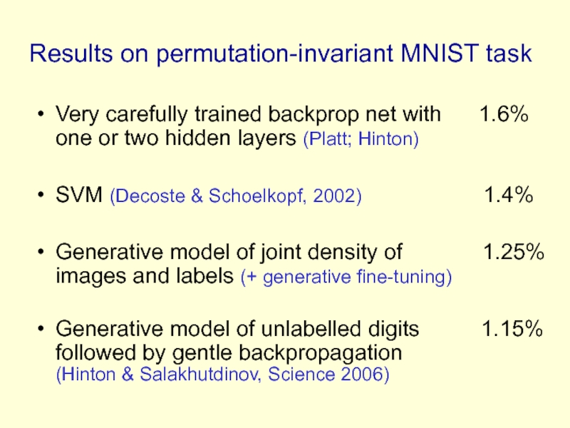
Слайд 56Results on permutation-invariant MNIST task
Very carefully trained backprop net with
SVM (Decoste & Schoelkopf, 2002) 1.4%
Generative model of joint density of 1.25% images and labels (+ generative fine-tuning)
Generative model of unlabelled digits 1.15% followed by gentle backpropagation (Hinton & Salakhutdinov, Science 2006)
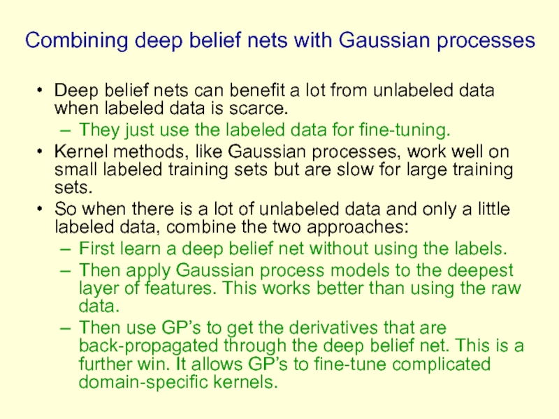
Слайд 57Combining deep belief nets with Gaussian processes
Deep belief nets can benefit
They just use the labeled data for fine-tuning.
Kernel methods, like Gaussian processes, work well on small labeled training sets but are slow for large training sets.
So when there is a lot of unlabeled data and only a little labeled data, combine the two approaches:
First learn a deep belief net without using the labels.
Then apply Gaussian process models to the deepest layer of features. This works better than using the raw data.
Then use GP’s to get the derivatives that are back-propagated through the deep belief net. This is a further win. It allows GP’s to fine-tune complicated domain-specific kernels.
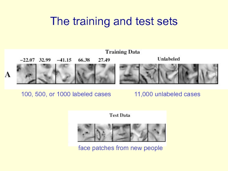
Слайд 59The training and test sets
11,000 unlabeled cases
100, 500, or 1000 labeled
face patches from new people
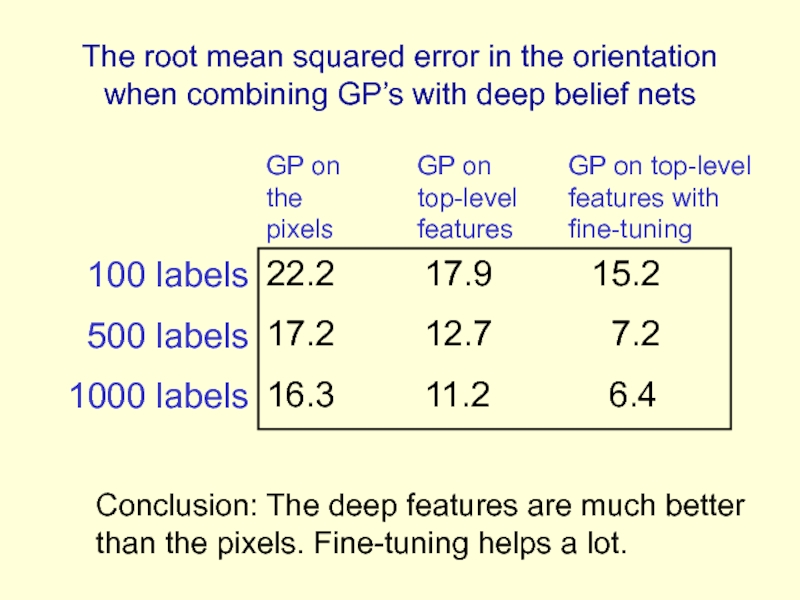
Слайд 60The root mean squared error in the orientation when combining GP’s
22.2 17.9 15.2
17.2 12.7 7.2
16.3 11.2 6.4
GP on the pixels
GP on top-level features
GP on top-level features with fine-tuning
100 labels
500 labels
1000 labels
Conclusion: The deep features are much better than the pixels. Fine-tuning helps a lot.
Слайд 61Modeling real-valued data
For images of digits it is possible to represent
We can treat intermediate values as the probability that the pixel is inked.
This will not work for real images.
In a real image, the intensity of a pixel is almost always almost exactly the average of the neighboring pixels.
Mean-field logistic units cannot represent precise intermediate values.
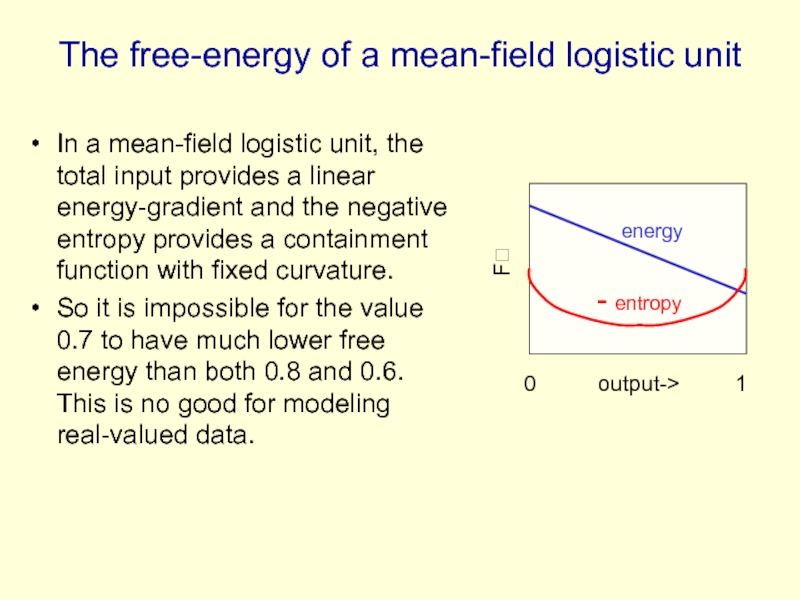
Слайд 62The free-energy of a mean-field logistic unit
In a mean-field logistic unit,
So it is impossible for the value 0.7 to have much lower free energy than both 0.8 and 0.6. This is no good for modeling real-valued data.
0 output-> 1
F?
energy
- entropy
Слайд 63An RBM with real-valued visible units
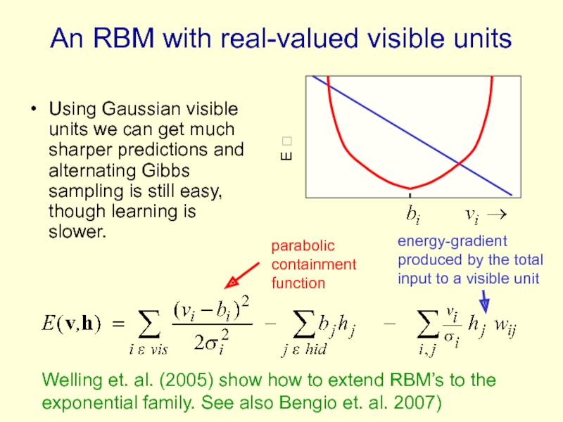
Using Gaussian visible units we can
E ?
energy-gradient produced by the total input to a visible unit
parabolic containment function
Welling et. al. (2005) show how to extend RBM’s to the exponential family. See also Bengio et. al. 2007)
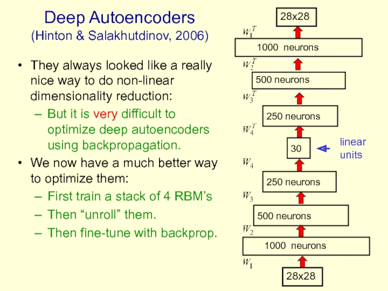
Слайд 64Deep Autoencoders
(Hinton & Salakhutdinov, 2006)
They always looked like a really nice
But it is very difficult to optimize deep autoencoders using backpropagation.
We now have a much better way to optimize them:
First train a stack of 4 RBM’s
Then “unroll” them.
Then fine-tune with backprop.
1000 neurons
500 neurons
500 neurons
250 neurons
250 neurons
30
1000 neurons
28x28
28x28
linear units
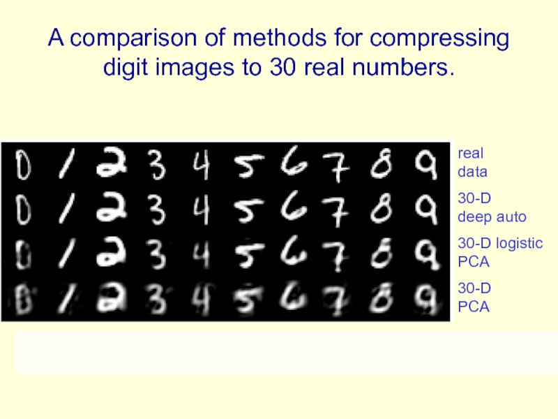
Слайд 65A comparison of methods for compressing digit images to 30 real
real data
30-D deep auto
30-D logistic PCA
30-D PCA
Слайд 66Do the 30-D codes found by the deep autoencoder preserve the
Take the 30-D activity patterns in the code layer and display them in 2-D using a new form of non-linear multi-dimensional scaling
The method is called UNI-SNE (Cook et. al. 2007).
It keeps similar patterns close together and tries to push dissimilar ones far apart.
Does the learning find the natural classes?
Слайд 68Retrieving documents that are similar to a query document
We can use
We start by converting each document into a “bag of words”. This a 2000 dimensional vector that contains the counts for each of the 2000 commonest words.
Слайд 69How to compress the count vector
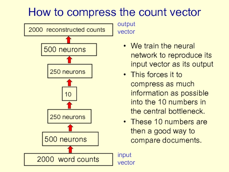
We train the neural network
This forces it to compress as much information as possible into the 10 numbers in the central bottleneck.
These 10 numbers are then a good way to compare documents.
2000 reconstructed counts
500 neurons
2000 word counts
500 neurons
250 neurons
250 neurons
10
input vector
output vector
Слайд 70Performance of the autoencoder at document retrieval
Train on bags of 2000
First train a stack of RBM’s. Then fine-tune with backprop.
Test on a separate 400,000 documents.
Pick one test document as a query. Rank order all the other test documents by using the cosine of the angle between codes.
Repeat this using each of the 400,000 test documents as the query (requires 0.16 trillion comparisons).
Plot the number of retrieved documents against the proportion that are in the same hand-labeled class as the query document.
Слайд 72
First compress all documents to 2 numbers using a type of
Слайд 73 First compress all documents
Слайд 74Finding binary codes for documents
Train an auto-encoder using 30 logistic units
During the fine-tuning stage, add noise to the inputs to the code units.
The “noise” vector for each training case is fixed. So we still get a deterministic gradient.
The noise forces their activities to become bimodal in order to resist the effects of the noise.
Then we simply round the activities of the 30 code units to 1 or 0.
2000 reconstructed counts
500 neurons
2000 word counts
500 neurons
250 neurons
250 neurons
30
noise
Слайд 75Semantic hashing: Using a deep autoencoder as a hash-function for finding
hash function
“supermarket search”
Слайд 76How good is a shortlist found this way?
We have only
A 20-D hypercube allows us to capture enough of the similarity structure of our document set.
The shortlist found using binary codes actually improves the precision-recall curves of TF-IDF.
Locality sensitive hashing (the fastest other method) is 50 times slower and has worse precision-recall curves.
Слайд 77Time series models
Inference is difficult in directed models of time series
It is hard to fit Dynamic Bayes Nets to high-dimensional sequences (e.g motion capture data).
So people tend to avoid distributed representations and use much weaker methods (e.g. HMM’s).
Слайд 78Time series models
If we really need distributed representations (which we nearly
Use an RBM for the interactions between hidden and visible variables. This ensures that the main source of information wants the posterior to be factorial.
Model short-range temporal information by allowing several previous frames to provide input to the hidden units and to the visible units.
This leads to a temporal module that can be stacked
So we can use greedy learning to learn deep models of temporal structure.
Слайд 79The conditional RBM model
(Sutskever & Hinton 2007)
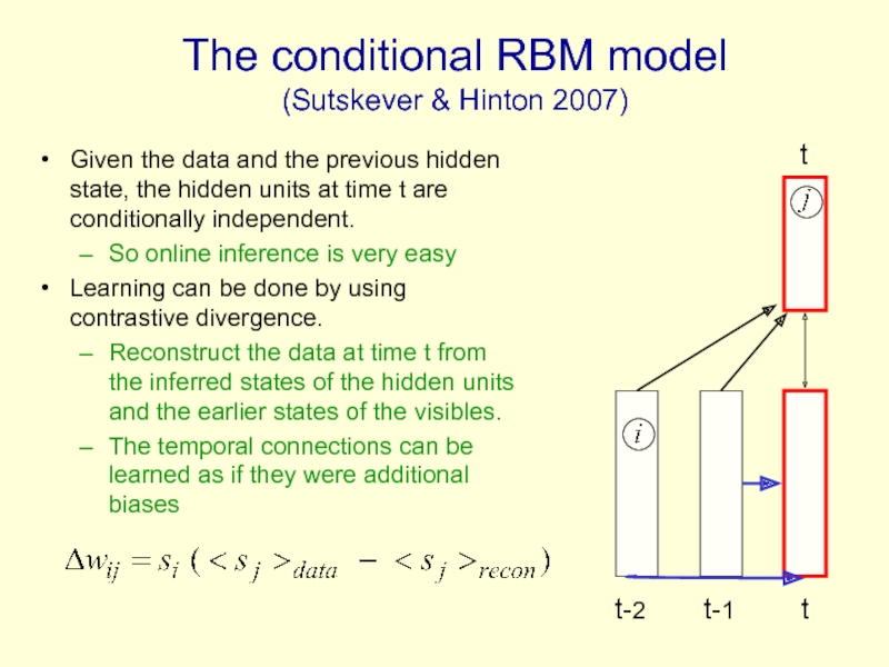
Given the data and
So online inference is very easy
Learning can be done by using contrastive divergence.
Reconstruct the data at time t from the inferred states of the hidden units and the earlier states of the visibles.
The temporal connections can be learned as if they were additional biases
t-2 t-1 t
t
Слайд 80Why the autoregressive connections do not cause problems
The autoregressive connections do
We know the initial state of the visible units, so we know the initial effect of the autoregressive connections.
It is not necessary for the reconstructions to be at equilibrium with the hidden units.
The important thing for contrastive divergence is to ensure the hiddens are in equilibrium with the visibles whenever statistics are measured.
Слайд 81Generating from a learned model
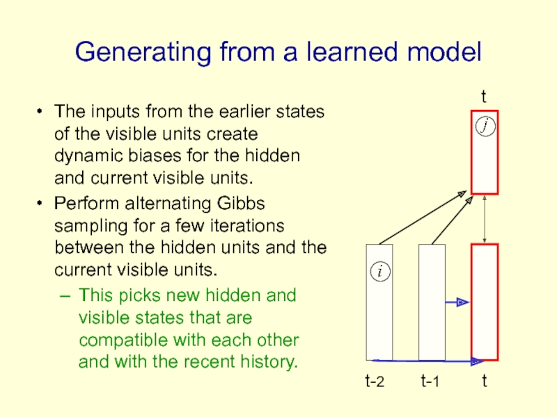
The inputs from the earlier states of
Perform alternating Gibbs sampling for a few iterations between the hidden units and the current visible units.
This picks new hidden and visible states that are compatible with each other and with the recent history.
t-2 t-1 t
t
Слайд 82Stacking temporal RBM’s
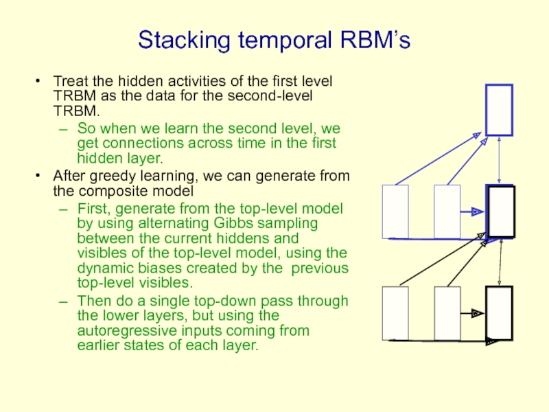
Treat the hidden activities of the first level TRBM
So when we learn the second level, we get connections across time in the first hidden layer.
After greedy learning, we can generate from the composite model
First, generate from the top-level model by using alternating Gibbs sampling between the current hiddens and visibles of the top-level model, using the dynamic biases created by the previous top-level visibles.
Then do a single top-down pass through the lower layers, but using the autoregressive inputs coming from earlier states of each layer.
Слайд 83An application to modeling motion capture data (Taylor, Roweis & Hinton,
Human motion can be captured by placing reflective markers on the joints and then using lots of infrared cameras to track the 3-D positions of the markers.
Given a skeletal model, the 3-D positions of the markers can be converted into the joint angles plus 6 parameters that describe the 3-D position and the roll, pitch and yaw of the pelvis.
We only represent changes in yaw because physics doesn’t care about its value and we want to avoid circular variables.
Слайд 84Modeling multiple types of motion
We can easily learn to model walking
This means we can share a lot of knowledge.
It should also make it much easier to learn nice transitions between walking and running.
In a switching mixture of dynamical systems its hard to get the latent variables to join up nicely when we switch from one system to another.
Because we can do online inference (slightly incorrectly), we can fill in missing markers in real time.
Слайд 86Generating the parts of an object
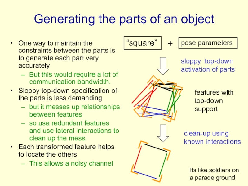
One way to maintain the
But this would require a lot of communication bandwidth.
Sloppy top-down specification of the parts is less demanding
but it messes up relationships between features
so use redundant features and use lateral interactions to clean up the mess.
Each transformed feature helps to locate the others
This allows a noisy channel
sloppy top-down activation of parts
clean-up using known interactions
pose parameters
features with top-down support
“square”
+
Its like soldiers on a parade ground
Слайд 87Semi-restricted Boltzmann Machines
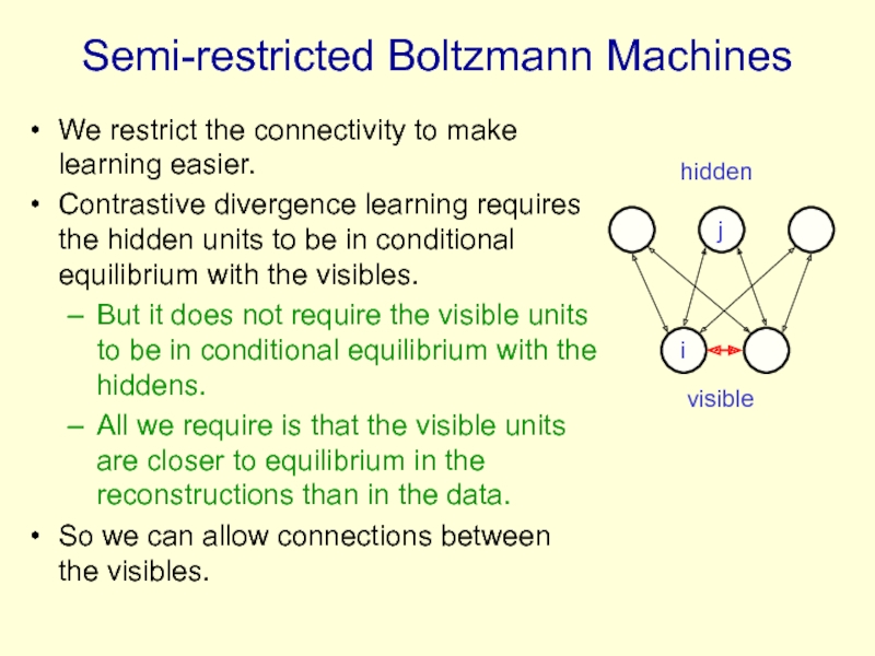
We restrict the connectivity to make learning easier.
Contrastive divergence
But it does not require the visible units to be in conditional equilibrium with the hiddens.
All we require is that the visible units are closer to equilibrium in the reconstructions than in the data.
So we can allow connections between the visibles.
hidden
i
j
visible
Слайд 88
Learning a semi-restricted Boltzmann Machine
i
j
i
j
t = 0
1. Start with a training vector on the visible units.
2. Update all of the hidden units in parallel
3. Repeatedly update all of the visible units in parallel using mean-field updates (with the hiddens fixed) to get a “reconstruction”.
4. Update all of the hidden units again.
reconstruction
data
k
i
i
k
k
k
update for a lateral weight
Слайд 89Learning in Semi-restricted Boltzmann Machines
Method 1: To form a reconstruction,
Method 2: Use “mean field” visible units that have real values. Update them all in parallel.
Use damping to prevent oscillations
total input to i
damping
Слайд 90Results on modeling natural image patches using a stack of RBM’s
Stack of RBM’s learned one at a time.
400 Gaussian visible units that see whitened image patches
Derived from 100,000 Van Hateren image patches, each 20x20
The hidden units are all binary.
The lateral connections are learned when they are the visible units of their RBM.
Reconstruction involves letting the visible units of each RBM settle using mean-field dynamics.
The already decided states in the level above determine the effective biases during mean-field settling.
Directed Connections
Directed Connections
Undirected Connections
400 Gaussian units
Hidden MRF with 2000 units
Hidden MRF with 500 units
1000 top-level units. No MRF.
Слайд 93A funny way to use an MRF
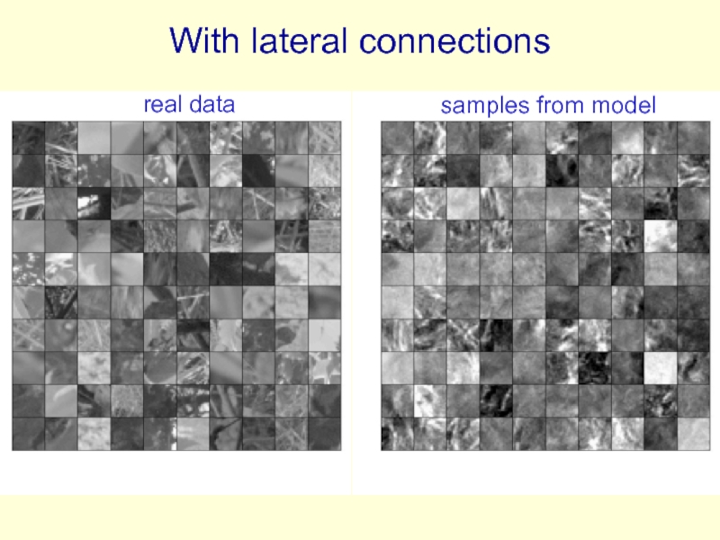
The lateral connections form an
The MRF is used during learning and generation.
The MRF is not used for inference.
This is a novel idea so vision researchers don’t like it.
The MRF enforces constraints. During inference, constraints do not need to be enforced because the data obeys them.
The constraints only need to be enforced during generation.
Unobserved hidden units cannot enforce constraints.
This requires lateral connections or observed descendants.
Слайд 94Why do we whiten data?
Images typically have strong pair-wise correlations.
Learning higher
Small changes in parameter values that improve the modeling of higher order statistics may be rejected because they form a slightly worse model of the much stronger pair-wise statistics.
So we often remove the second-order statistics before trying to learn the higher-order statistics.
Слайд 95Whitening the learning signal instead of the data
Contrastive divergence learning can
The lateral connections model the second order statistics
If a pixel can be reconstructed correctly using second order statistics, its will be the same in the reconstruction as in the data.
The hidden units can then focus on modeling high-order structure that cannot be predicted by the lateral connections.
For example, a pixel close to an edge, where interpolation from nearby pixels causes incorrect smoothing.
Слайд 96Towards a more powerful, multi-linear stackable learning module
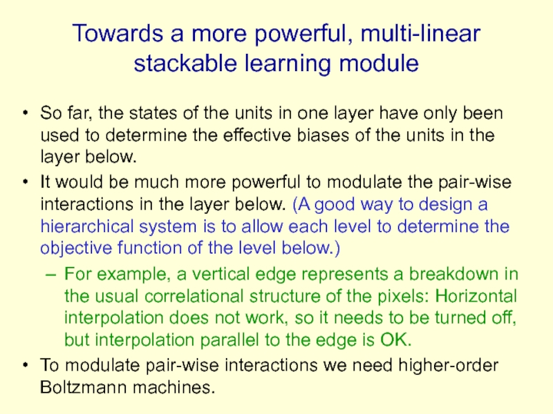
So far, the states
It would be much more powerful to modulate the pair-wise interactions in the layer below. (A good way to design a hierarchical system is to allow each level to determine the objective function of the level below.)
For example, a vertical edge represents a breakdown in the usual correlational structure of the pixels: Horizontal interpolation does not work, so it needs to be turned off, but interpolation parallel to the edge is OK.
To modulate pair-wise interactions we need higher-order Boltzmann machines.
Слайд 97Higher order Boltzmann machines (Sejnowski, ~1986)
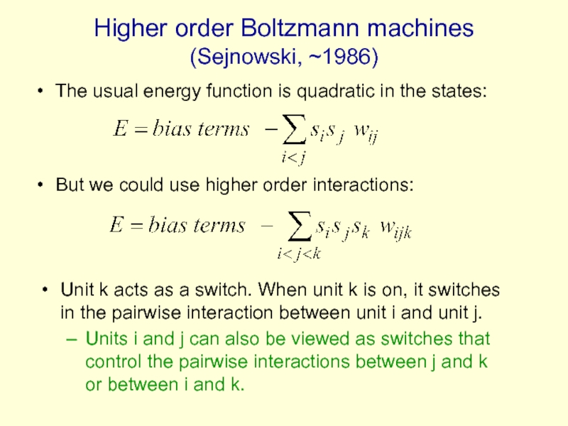
The usual energy function is quadratic
But we could use higher order interactions:
Unit k acts as a switch. When unit k is on, it switches in the pairwise interaction between unit i and unit j.
Units i and j can also be viewed as switches that control the pairwise interactions between j and k or between i and k.
Слайд 98A picture of a conditional,
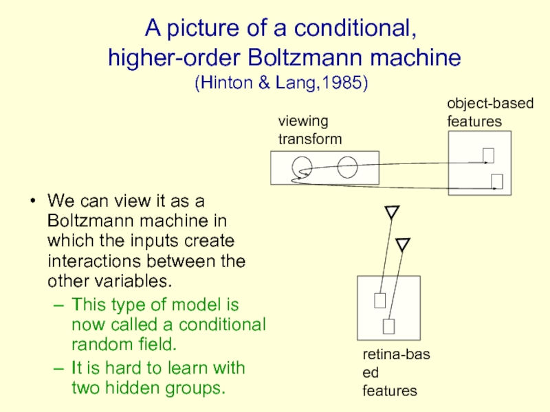
higher-order Boltzmann machine
(Hinton & Lang,1985)
retina-based
object-based features
viewing transform
We can view it as a Boltzmann machine in which the inputs create interactions between the other variables.
This type of model is now called a conditional random field.
It is hard to learn with two hidden groups.
Слайд 99Using conditional higher-order Boltzmann machines to model image transformations (Memisevic and
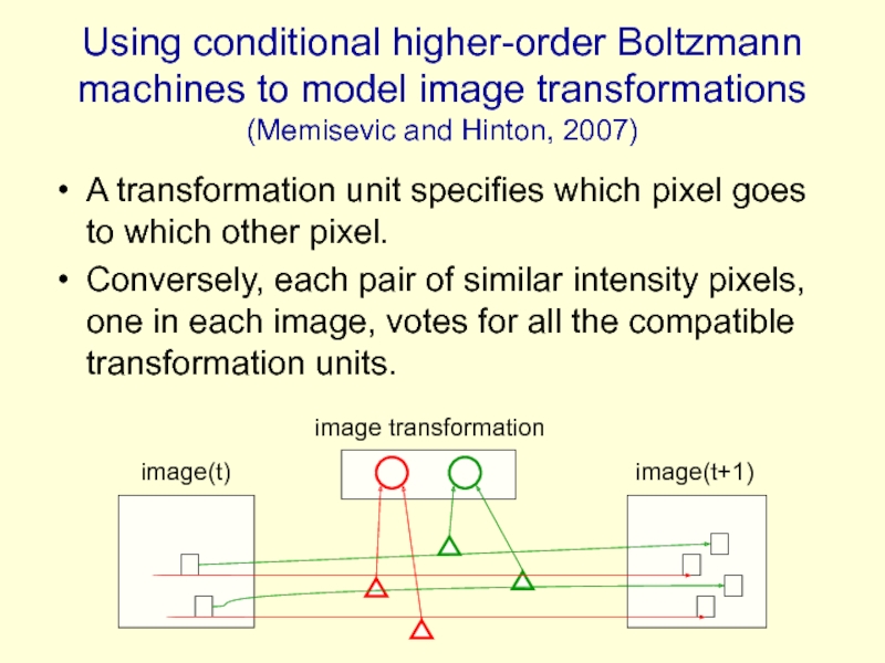
A transformation unit specifies which pixel goes to which other pixel.
Conversely, each pair of similar intensity pixels, one in each image, votes for all the compatible transformation units.
image(t)
image(t+1)
image transformation
Слайд 100Readings on deep belief nets
A reading list (that is still being
www.cs.toronto.edu/~hinton/csc2515/deeprefs.html
