- Главная
- Разное
- Дизайн
- Бизнес и предпринимательство
- Аналитика
- Образование
- Развлечения
- Красота и здоровье
- Финансы
- Государство
- Путешествия
- Спорт
- Недвижимость
- Армия
- Графика
- Культурология
- Еда и кулинария
- Лингвистика
- Английский язык
- Астрономия
- Алгебра
- Биология
- География
- Детские презентации
- Информатика
- История
- Литература
- Маркетинг
- Математика
- Медицина
- Менеджмент
- Музыка
- МХК
- Немецкий язык
- ОБЖ
- Обществознание
- Окружающий мир
- Педагогика
- Русский язык
- Технология
- Физика
- Философия
- Химия
- Шаблоны, картинки для презентаций
- Экология
- Экономика
- Юриспруденция
Cmpe 466 computer graphics. Graphics output primitives. (Chapter 4) презентация
Содержание
- 1. Cmpe 466 computer graphics. Graphics output primitives. (Chapter 4)
- 2. Output primitives and reference frames Output primitives
- 3. Screen coordinates Screen coordinates (integers): Locations on
- 4. Specifying a 2D WC reference frame Figure
- 5. OpenGL point functions glBegin (GL_POINTS);
- 6. OpenGL point functions: alternative code int point1
- 7. More on point functions Specifying positions in
- 8. OpenGL line functions Figure 4-4 Line
- 9. Polygon Fill Areas Figure 4-8 A
- 10. Identifying concave polygons Figure 4-9 Identifying
- 11. Splitting concave polygons: vector method Form the
- 12. Splitting example Figure 4-10 Splitting a concave polygon using the vector method.
- 13. Splitting polygons
- 14. Splitting a convex polygon into a set
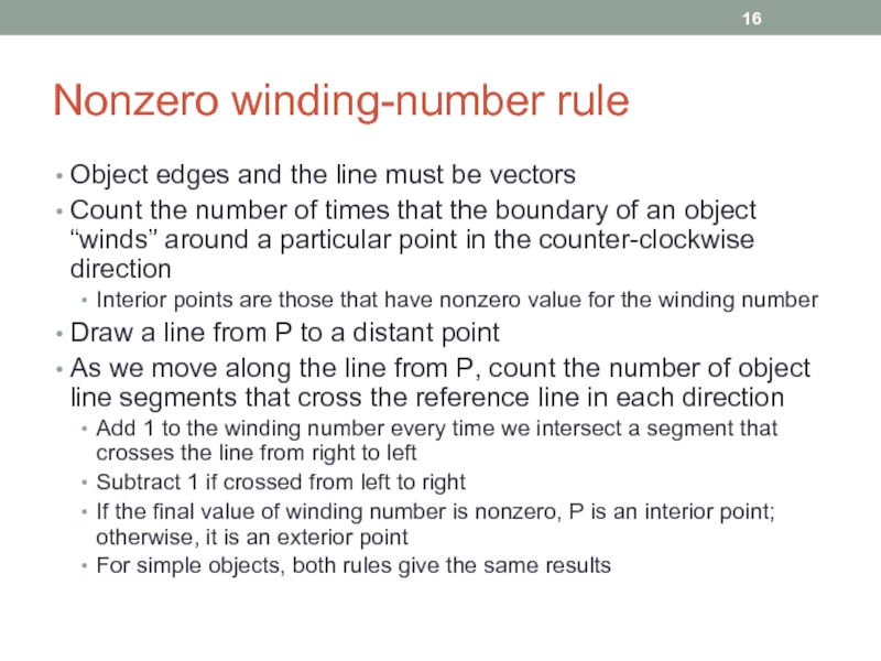
- 15. Inside-outside tests Odd-even rule Draw a line
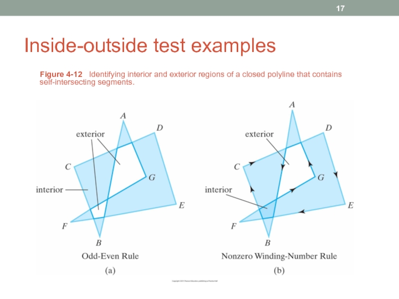
- 16. Nonzero winding-number rule Object edges and the
- 17. Inside-outside test examples Figure 4-12 Identifying
- 18. Variations of nonzero winding-number rule Figure 4-13
- 19. Variations of nonzero winding-number rule Figure 4-14
- 20. Variations of nonzero winding-number rule Figure 4-15
- 21. Polygon tables Figure 4-16 Geometric data-table
- 22. Plane equations Often, information about spatial orientation
- 23. Solutions to plane equations We obtain A,
- 24. Solutions Then
- 25. Front and back polygon faces Faces can
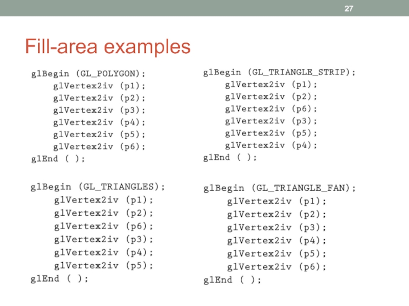
- 26. OpenGL polygon fill-area functions Figure 4-22
- 27. Fill-area examples
- 28. Quadrilateral fill-areas Figure 4-23 Displaying quadrilateral
- 29. A complex scene might require hundreds or
- 30. Using a vertex array Figure 4-25
- 31. Display lists const double TWO_PI = 6.2831853;
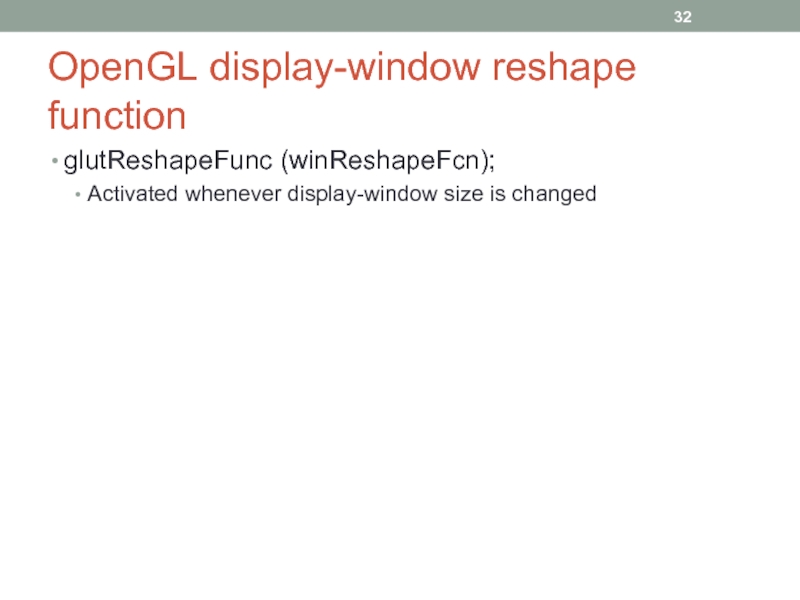
- 32. OpenGL display-window reshape function glutReshapeFunc (winReshapeFcn); Activated whenever display-window size is changed
Слайд 1CMPE 466
COMPUTER GRAPHICS
Chapter 4
Graphics Output Primitives
Instructor: D. Arifler
Material based on
- Computer
- Fundamentals of Computer Graphics, Third Edition by by Peter Shirley and Steve Marschner
Слайд 2Output primitives and reference frames
Output primitives are functions that we use
World-coordinate (WC) reference frame describes objects in the picture by giving their geometric specs in terms of positions in WC
Scene info is processed by viewing routines
These routines identify visible surfaces
Scan conversion stores info about the scene at the appropriate locations in frame buffer
Finally, objects are displayed on output device
Слайд 3Screen coordinates
Screen coordinates (integers): Locations on a video monitor
Coordinates correspond to
Pixel positions: Scan line number (y-value), column number (x-value along a scan line)
Hardware processes, such as screen refreshing, typically address pixel positions with respect to the top-left corner of the screen
With software commands, we can set up any convenient reference frame for screen positions
Слайд 4Specifying a 2D WC reference frame
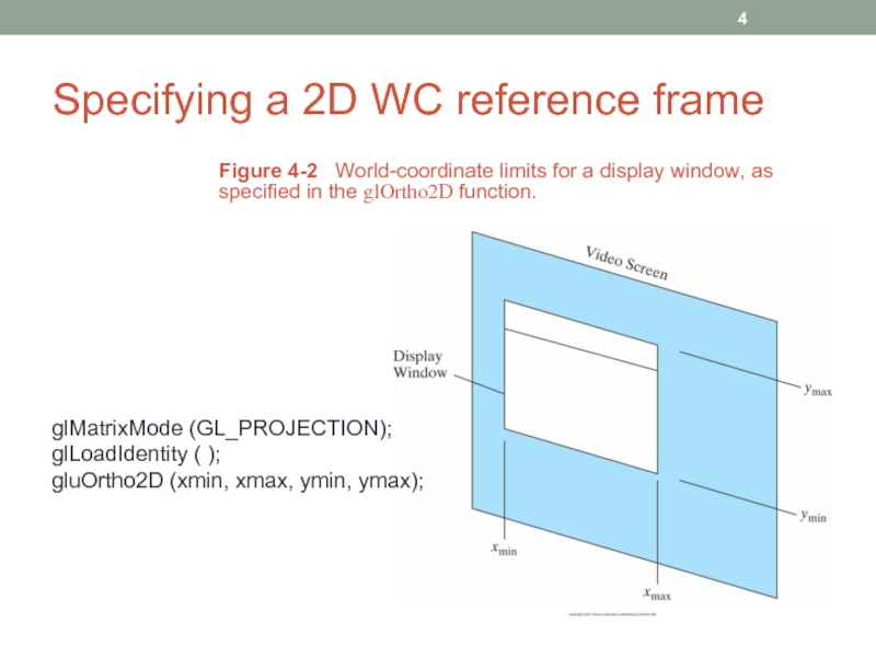
Figure 4-2 World-coordinate limits for
glMatrixMode (GL_PROJECTION);
glLoadIdentity ( );
gluOrtho2D (xmin, xmax, ymin, ymax);
Слайд 5OpenGL point functions
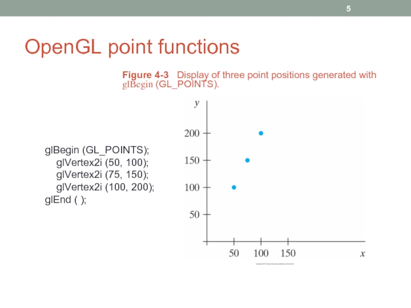
glBegin (GL_POINTS);
glVertex2i (50, 100);
glVertex2i (75,
glVertex2i (100, 200);
glEnd ( );
Figure 4-3 Display of three point positions generated with glBegin (GL_POINTS).
Слайд 6OpenGL point functions: alternative code
int point1 [ ] = {50, 100};
int
int point3 [ ] = {100, 200};
…
glBegin (GL_POINTS);
glVertex2iv (point1);
glVertex2iv (point2);
glVertex2iv (point3);
glEnd ( );
Figure 4-3 Display of three point positions generated with glBegin (GL_POINTS).
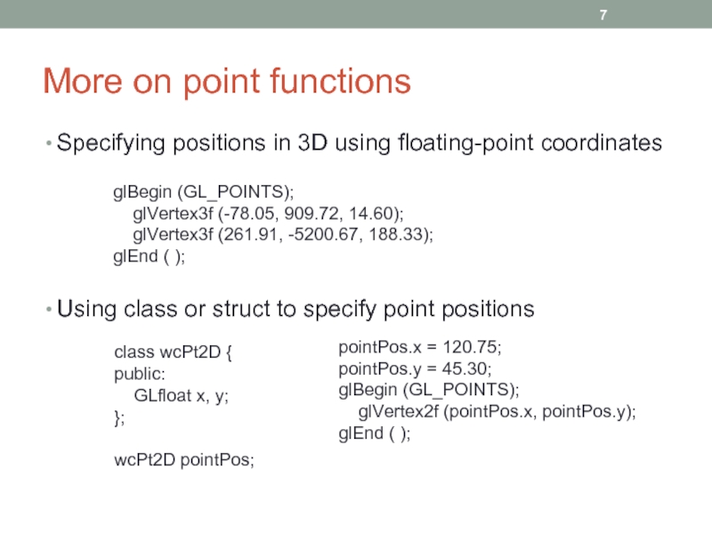
Слайд 7More on point functions
Specifying positions in 3D using floating-point coordinates
Using class
glBegin (GL_POINTS);
glVertex3f (-78.05, 909.72, 14.60);
glVertex3f (261.91, -5200.67, 188.33);
glEnd ( );
class wcPt2D {
public:
GLfloat x, y;
};
wcPt2D pointPos;
pointPos.x = 120.75;
pointPos.y = 45.30;
glBegin (GL_POINTS);
glVertex2f (pointPos.x, pointPos.y);
glEnd ( );
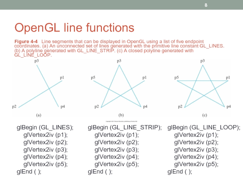
Слайд 8OpenGL line functions
Figure 4-4 Line segments that can be displayed
glBegin (GL_LINES);
glVertex2iv (p1);
glVertex2iv (p2);
glVertex2iv (p3);
glVertex2iv (p4);
glVertex2iv (p5);
glEnd ( );
glBegin (GL_LINE_STRIP);
glVertex2iv (p1);
glVertex2iv (p2);
glVertex2iv (p3);
glVertex2iv (p4);
glVertex2iv (p5);
glEnd ( );
glBegin (GL_LINE_LOOP);
glVertex2iv (p1);
glVertex2iv (p2);
glVertex2iv (p3);
glVertex2iv (p4);
glVertex2iv (p5);
glEnd ( );
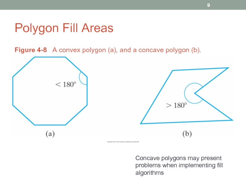
Слайд 9Polygon Fill Areas
Figure 4-8 A convex polygon (a), and a
Concave polygons may present problems when implementing fill algorithms
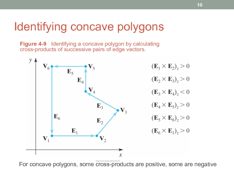
Слайд 10Identifying concave polygons
Figure 4-9 Identifying a concave polygon by calculating
For concave polygons, some cross-products are positive, some are negative
Слайд 11Splitting concave polygons: vector method
Form the edge vectors Ek=Vk+1 - Vk
Calculate
Use the cross-product test to identify concave polygons
If any cross-product has a negative z-component, the polygon is concave and we can split it along the line of the first edge vector in the cross-product pair
Слайд 14Splitting a convex polygon into a set of triangles
Triangles make several
Define any sequence of three consecutive vertices to be a new polygon (triangle)
Delete the middle triangle vertex from the original vertex list
Apply the same procedure to the modified list to strip off another triangle
Continue until the original polygon is reduced to just three vertices (the last triangle)
Слайд 15Inside-outside tests
Odd-even rule
Draw a line from any position P to a
Count the number of line segment crossings along this line
If odd, P is an interior point
Otherwise, P is an exterior point
Note that the line must not intersect any line segment end-points
Слайд 16Nonzero winding-number rule
Object edges and the line must be vectors
Count the
Interior points are those that have nonzero value for the winding number
Draw a line from P to a distant point
As we move along the line from P, count the number of object line segments that cross the reference line in each direction
Add 1 to the winding number every time we intersect a segment that crosses the line from right to left
Subtract 1 if crossed from left to right
If the final value of winding number is nonzero, P is an interior point; otherwise, it is an exterior point
For simple objects, both rules give the same results
Слайд 17Inside-outside test examples
Figure 4-12 Identifying interior and exterior regions of
Слайд 18Variations of nonzero winding-number rule
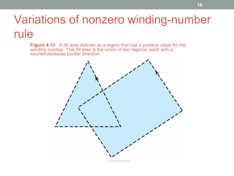
Figure 4-13 A fill area defined
Слайд 19Variations of nonzero winding-number rule
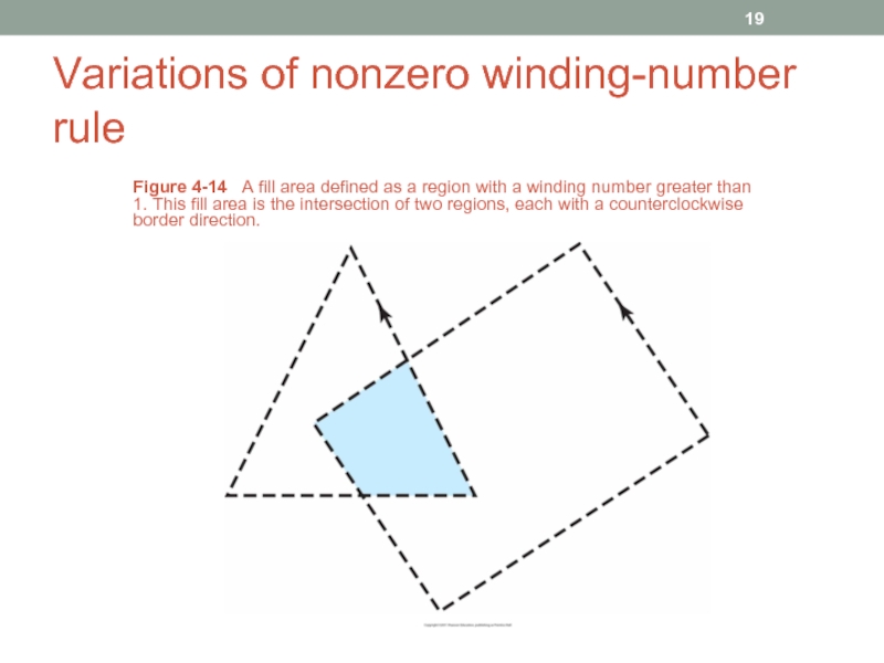
Figure 4-14 A fill area defined
Слайд 20Variations of nonzero winding-number rule
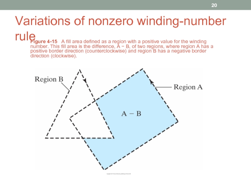
Figure 4-15 A fill area defined
Слайд 21Polygon tables
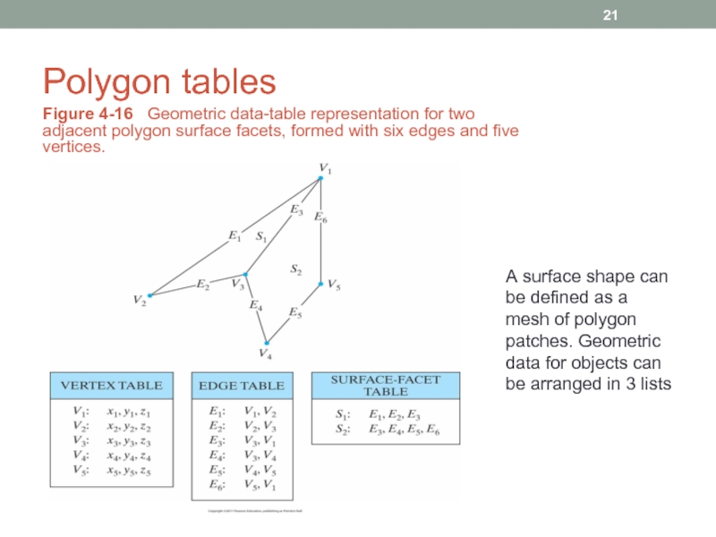
Figure 4-16 Geometric data-table representation for two adjacent polygon
A surface shape can be defined as a mesh of polygon patches. Geometric
data for objects can be arranged in 3 lists
Слайд 22Plane equations
Often, information about spatial orientation of surface components is needed
This
Each polygon in a scene is contained within a plane of infinite extent
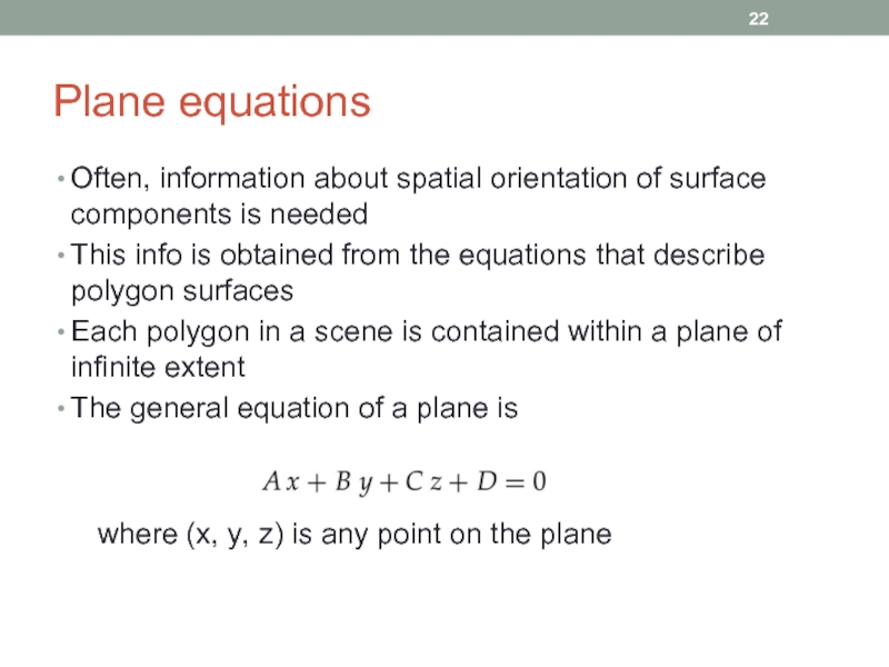
The general equation of a plane is
where (x, y, z) is any point on the plane
Слайд 23Solutions to plane equations
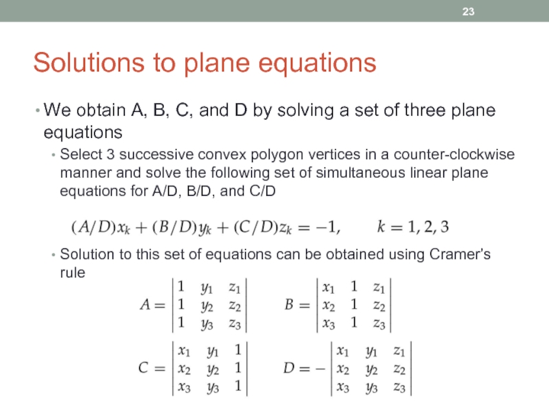
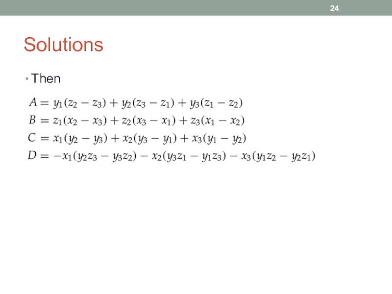
We obtain A, B, C, and D by
Select 3 successive convex polygon vertices in a counter-clockwise manner and solve the following set of simultaneous linear plane equations for A/D, B/D, and C/D
Solution to this set of equations can be obtained using Cramer’s rule
Слайд 25Front and back polygon faces
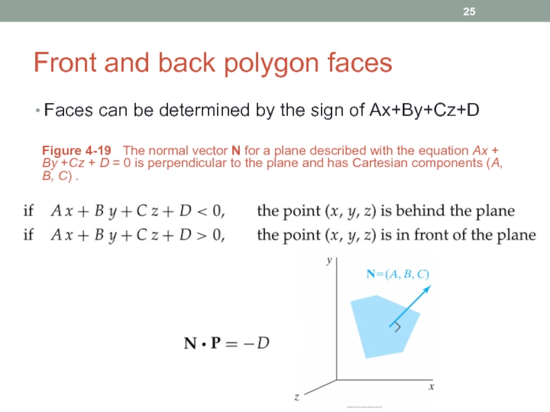
Faces can be determined by the sign
Figure 4-19 The normal vector N for a plane described with the equation Ax + By +Cz + D = 0 is perpendicular to the plane and has Cartesian components (A, B, C) .
Слайд 26OpenGL polygon fill-area functions
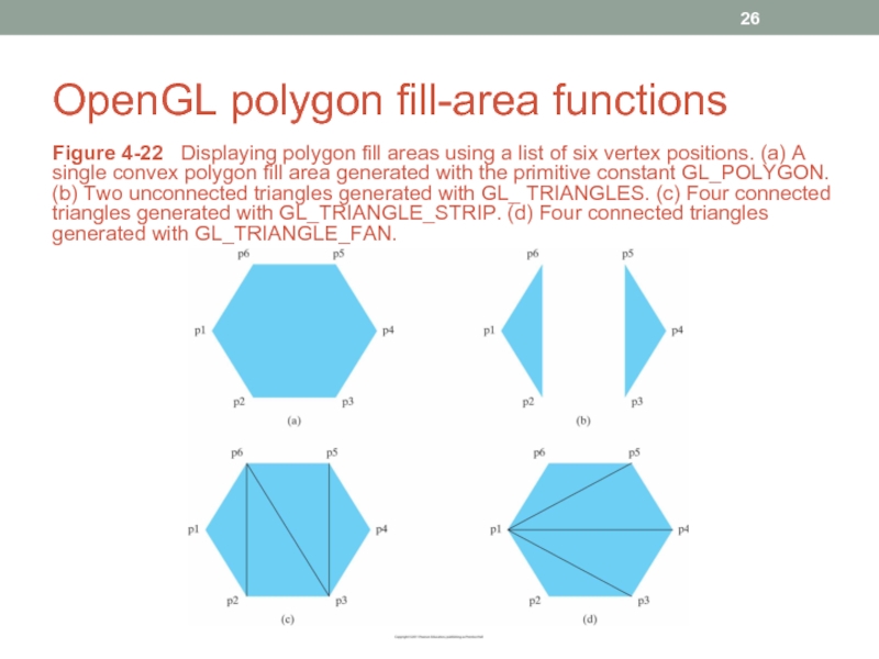
Figure 4-22 Displaying polygon fill areas using
Слайд 28Quadrilateral fill-areas
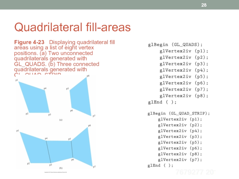
Figure 4-23 Displaying quadrilateral fill areas using a list
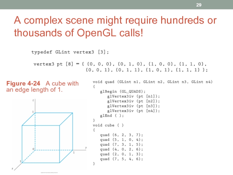
Слайд 29A complex scene might require hundreds or thousands of OpenGL calls!
Figure
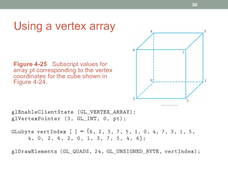
Слайд 30Using a vertex array
Figure 4-25 Subscript values for array pt
}
{
Слайд 31Display lists
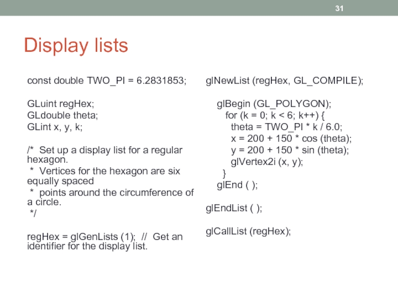
const double TWO_PI = 6.2831853;
GLuint regHex;
GLdouble theta;
GLint x, y, k;
/*
* Vertices for the hexagon are six equally spaced
* points around the circumference of a circle.
*/
regHex = glGenLists (1); // Get an identifier for the display list.
glNewList (regHex, GL_COMPILE);
glBegin (GL_POLYGON);
for (k = 0; k < 6; k++) {
theta = TWO_PI * k / 6.0;
x = 200 + 150 * cos (theta);
y = 200 + 150 * sin (theta);
glVertex2i (x, y);
}
glEnd ( );
glEndList ( );
glCallList (regHex);
![OpenGL point functions: alternative codeint point1 [ ] = {50, 100};int point2 [ ] =](/img/tmb/2/127218/d932bceb760710d59a3fb86d9db36404-800x.jpg)
