- Главная
- Разное
- Дизайн
- Бизнес и предпринимательство
- Аналитика
- Образование
- Развлечения
- Красота и здоровье
- Финансы
- Государство
- Путешествия
- Спорт
- Недвижимость
- Армия
- Графика
- Культурология
- Еда и кулинария
- Лингвистика
- Английский язык
- Астрономия
- Алгебра
- Биология
- География
- Детские презентации
- Информатика
- История
- Литература
- Маркетинг
- Математика
- Медицина
- Менеджмент
- Музыка
- МХК
- Немецкий язык
- ОБЖ
- Обществознание
- Окружающий мир
- Педагогика
- Русский язык
- Технология
- Физика
- Философия
- Химия
- Шаблоны, картинки для презентаций
- Экология
- Экономика
- Юриспруденция
Clustering. DBScan презентация
Содержание
- 1. Clustering. DBScan
- 2. Compare results K-means: http://www.naftaliharris.com/blog/visualizing-k-means-clustering/ (I’ll
- 3. DBSCAN Density-based spatial clustering of applications with
- 4. Preliminary Consider a set of points in
- 5. Preliminary If p is a core point,
- 6. Preliminary Two points p and q are
- 7. Example In this
- 8. Algorithm DBSCAN requires two parameters: ε (eps)
- 9. Algorithm If a point is found to
- 10. Main procedure
- 11. Procedure expandCluster
- 12. Procedure regionQuery
- 13. Note The algorithm can be simplified by
- 14. Complexity DBSCAN visits each point of the
- 15. Parameter estimation (minPts) Ideally, minPts is the
- 16. Parameter estimation (ε) If ε is chosen
- 17. Advantages DBSCAN does not require to specify
- 18. Disadvantages DBSCAN is not entirely deterministic: border
- 19. DBScan and DBMS Nothing…
- 20. Task 5 Generate 3-4 areas (2D or
Слайд 2
Compare results
K-means:
http://www.naftaliharris.com/blog/visualizing-k-means-clustering/
(I’ll choose -> Gaussian Mixture, Smiley Face)
DBScan:
http://www.naftaliharris.com/blog/visualizing-dbscan-clustering/
(Gaussian Mixture, Smiley Face)
Слайд 3DBSCAN
Density-based spatial clustering of applications with noise (DBSCAN) is a
data clustering algorithm proposed by Martin Ester, Hans-Peter Kriegel, Jörg Sander and Xiaowei Xu in 1996. It is a density-based clustering algorithm: given a set of points in some space, it groups together points that are closely packed together (points with many nearby neighbors), marking as outliers points that lie alone in low-density regions (whose nearest neighbors are too far away). DBSCAN is one of the most common clustering algorithms and also most cited in scientific literature.
In 2014, the algorithm was awarded the test of time award (an award given to algorithms which have received substantial attention in theory and practice) at the leading data mining conference, KDD.
In 2014, the algorithm was awarded the test of time award (an award given to algorithms which have received substantial attention in theory and practice) at the leading data mining conference, KDD.
Слайд 4Preliminary
Consider a set of points in some space to be clustered.
For the purpose of DBSCAN clustering, the points are classified as core points, (density-) reachable points and outliers (noise), as follows:
A point p is a core point if at least minPts points are within distance ε of it, and those points are said to be directly reachable from p.
A point q is reachable from p if there is a path p1, ..., pn with p1 = p and pn = q, where each pi+1 is directly reachable from pi (so all the points on the path must be core points, with the possible exception of q).
All points not reachable from any other point are outliers.
Слайд 5Preliminary
If p is a core point, then it forms a cluster
together with all points
(core or non-core) that are reachable from it. Each cluster contains at
least one core point; non-core points can be part of a cluster, but they
form its "edge", since they cannot be used to reach more points.
(core or non-core) that are reachable from it. Each cluster contains at
least one core point; non-core points can be part of a cluster, but they
form its "edge", since they cannot be used to reach more points.
Слайд 6Preliminary
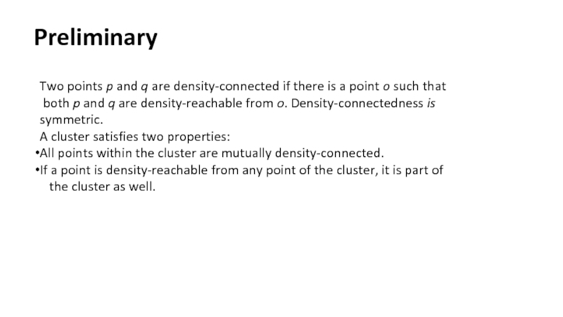
Two points p and q are density-connected if there is a
point o such that
both p and q are density-reachable from o. Density-connectedness is
symmetric.
A cluster satisfies two properties:
All points within the cluster are mutually density-connected.
If a point is density-reachable from any point of the cluster, it is part of
the cluster as well.
both p and q are density-reachable from o. Density-connectedness is
symmetric.
A cluster satisfies two properties:
All points within the cluster are mutually density-connected.
If a point is density-reachable from any point of the cluster, it is part of
the cluster as well.
Слайд 7Example
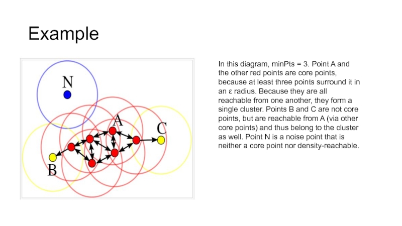
In this diagram, minPts = 3. Point A and
the other red points are core points, because at least three points surround it in an ε radius. Because they are all reachable from one another, they form a single cluster. Points B and C are not core points, but are reachable from A (via other core points) and thus belong to the cluster as well. Point N is a noise point that is neither a core point nor density-reachable.
Слайд 8Algorithm
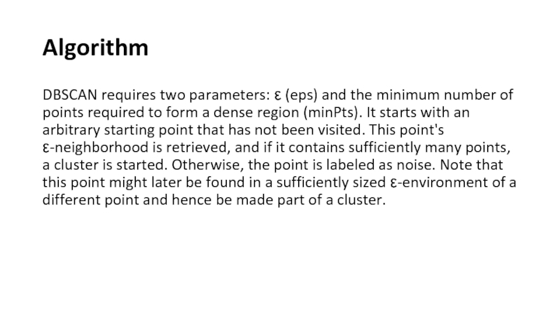
DBSCAN requires two parameters: ε (eps) and the minimum number of
points required to form a dense region (minPts). It starts with an arbitrary starting point that has not been visited. This point's ε-neighborhood is retrieved, and if it contains sufficiently many points, a cluster is started. Otherwise, the point is labeled as noise. Note that this point might later be found in a sufficiently sized ε-environment of a different point and hence be made part of a cluster.
Слайд 9Algorithm
If a point is found to be a dense part of
a cluster, its ε-neighborhood is also part of that cluster. Hence, all points that are found within the ε-neighborhood are added, as is their own ε-neighborhood when they are also dense. This process continues until the density-connected cluster is completely found. Then, a new unvisited point is retrieved and processed, leading to the discovery of a further cluster or noise.
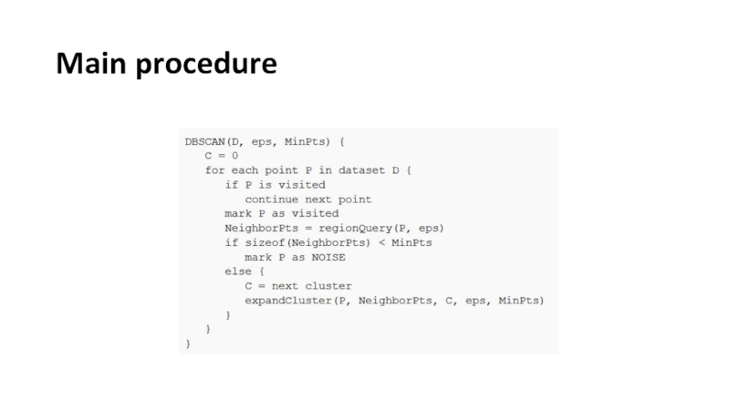
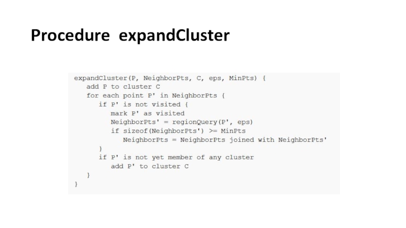
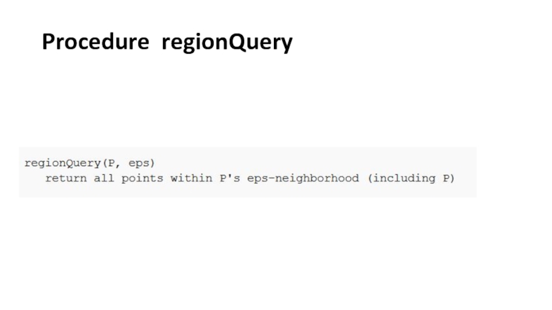
The algorithm can be expressed as follows, in pseudocode following the original published nomenclature.
The algorithm can be expressed as follows, in pseudocode following the original published nomenclature.
Слайд 13Note
The algorithm can be simplified by merging the per-point "has been
visited" and "belongs to cluster C" logic, as well as by inlining the contents of the "expandCluster" subroutine, which is only called from one place. These simplifications have been omitted from the above pseudocode in order to reflect the originally published version. Additionally, the regionQuery function need not return P in the list of points to be visited, as long as it is otherwise still counted in the local density estimate.
Слайд 14Complexity
DBSCAN visits each point of the database, possibly multiple times (e.g.,
as candidates to different clusters). For practical considerations, however, the time complexity is mostly governed by the number of regionQuery invocations. DBSCAN executes exactly one such query for each point, and if an indexing structure is used that executes a neighborhood query in O(log n), an overall average runtime complexity of O(n log n) is obtained (if parameter ε is chosen in a meaningful way, i.e. such that on average only O(log n) points are returned). Without the use of an accelerating index structure, or on degenerated data (e.g. all points within a distance less than ε), the worst case run time complexity remains O(n²).
Слайд 15Parameter estimation (minPts)
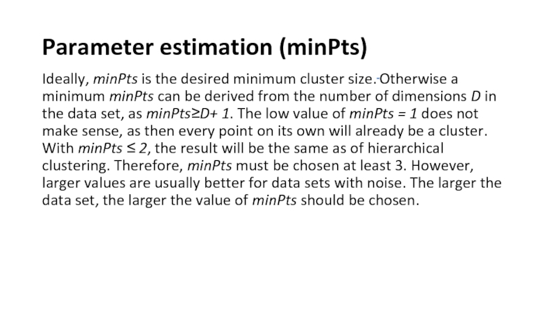
Ideally, minPts is the desired minimum cluster size. Otherwise
a minimum minPts can be derived from the number of dimensions D in the data set, as minPts≥D+ 1. The low value of minPts = 1 does not make sense, as then every point on its own will already be a cluster. With minPts ≤ 2, the result will be the same as of hierarchical clustering. Therefore, minPts must be chosen at least 3. However, larger values are usually better for data sets with noise. The larger the data set, the larger the value of minPts should be chosen.
Слайд 16Parameter estimation (ε)
If ε is chosen much too small, a large
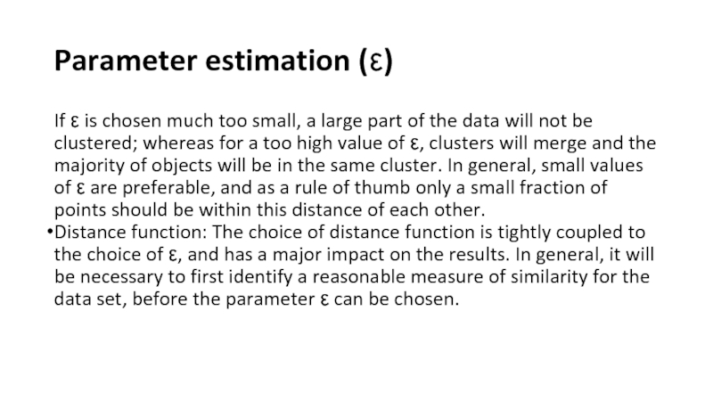
part of the data will not be clustered; whereas for a too high value of ε, clusters will merge and the majority of objects will be in the same cluster. In general, small values of ε are preferable, and as a rule of thumb only a small fraction of points should be within this distance of each other.
Distance function: The choice of distance function is tightly coupled to the choice of ε, and has a major impact on the results. In general, it will be necessary to first identify a reasonable measure of similarity for the data set, before the parameter ε can be chosen.
Distance function: The choice of distance function is tightly coupled to the choice of ε, and has a major impact on the results. In general, it will be necessary to first identify a reasonable measure of similarity for the data set, before the parameter ε can be chosen.
Слайд 17Advantages
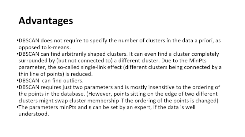
DBSCAN does not require to specify the number of clusters in
the data a priori, as opposed to k-means.
DBSCAN can find arbitrarily shaped clusters. It can even find a cluster completely surrounded by (but not connected to) a different cluster. Due to the MinPts parameter, the so-called single-link effect (different clusters being connected by a thin line of points) is reduced.
DBSCAN can find outliers.
DBSCAN requires just two parameters and is mostly insensitive to the ordering of the points in the database. (However, points sitting on the edge of two different clusters might swap cluster membership if the ordering of the points is changed)
The parameters minPts and ε can be set by an expert, if the data is well understood.
Слайд 18Disadvantages
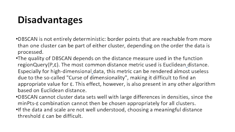
DBSCAN is not entirely deterministic: border points that are reachable from
more than one cluster can be part of either cluster, depending on the order the data is processed.
The quality of DBSCAN depends on the distance measure used in the function regionQuery(P,ε). The most common distance metric used is Euclidean distance. Especially for high-dimensional data, this metric can be rendered almost useless due to the so-called "Curse of dimensionality", making it difficult to find an appropriate value for ε. This effect, however, is also present in any other algorithm based on Euclidean distance.
DBSCAN cannot cluster data sets well with large differences in densities, since the minPts-ε combination cannot then be chosen appropriately for all clusters.
If the data and scale are not well understood, choosing a meaningful distance threshold ε can be difficult.
Слайд 20Task 5
Generate 3-4 areas (2D or 3D).
Create an application and show
the areas.
Realize DBScan algorithm and cluster the areas.
Show the result of clustering (paint the clusters with different
colors).
Realize DBScan algorithm and cluster the areas.
Show the result of clustering (paint the clusters with different
colors).
