- Главная
- Разное
- Дизайн
- Бизнес и предпринимательство
- Аналитика
- Образование
- Развлечения
- Красота и здоровье
- Финансы
- Государство
- Путешествия
- Спорт
- Недвижимость
- Армия
- Графика
- Культурология
- Еда и кулинария
- Лингвистика
- Английский язык
- Астрономия
- Алгебра
- Биология
- География
- Детские презентации
- Информатика
- История
- Литература
- Маркетинг
- Математика
- Медицина
- Менеджмент
- Музыка
- МХК
- Немецкий язык
- ОБЖ
- Обществознание
- Окружающий мир
- Педагогика
- Русский язык
- Технология
- Физика
- Философия
- Химия
- Шаблоны, картинки для презентаций
- Экология
- Экономика
- Юриспруденция
Assumption of homoscedasticty презентация
Содержание
- 1. Assumption of homoscedasticty
- 2. Assumption of Homoscedasticity Homoscedasticity refers to the
- 3. Evaluating homoscedasticity Homoscedasticity is evaluated for
- 4. Transformations When the assumption of homoscedasticity is
- 5. When transformations do not work When none
- 6. Problem 1 In the dataset GSS2000.sav, is
- 7. Request a boxplot The boxplot provides a
- 8. Specify the type of boxplot First, click
- 9. Specify the dependent variable First, click on
- 10. Specify the independent variable First, click on
- 11. Complete the request for the boxplot To
- 12. The boxplot Each red box shows the
- 13. Request the test for homogeneity of variance
- 14. Specify the independent variable First, click on
- 15. Specify the dependent variable First, click on
- 16. The homogeneity of variance test is an
- 17. Specify the homogeneity of variance test First,
- 18. Complete the request for output Click on
- 19. Interpreting the homogeneity of variance test The
- 20. The assumption of homoscedasticity script An SPSS
- 21. Selecting the assumption of homoscedasticity script First,
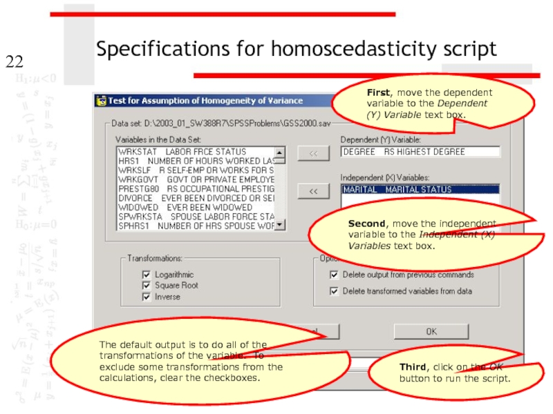
- 22. Specifications for homoscedasticity script The default output
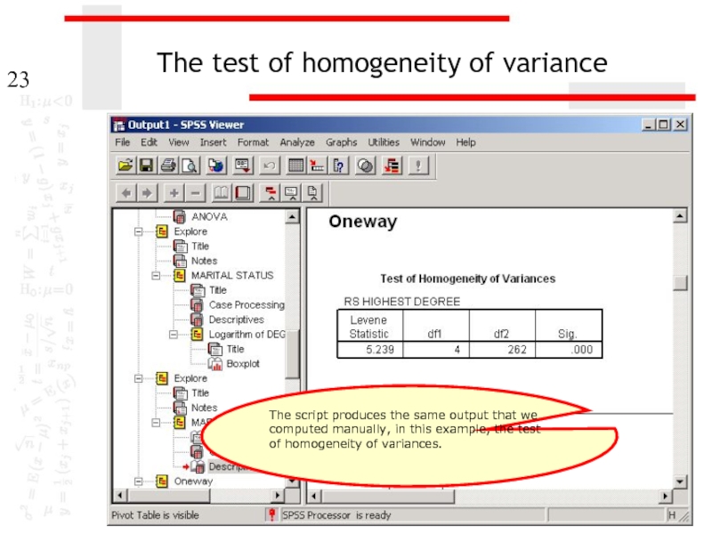
- 23. The test of homogeneity of variance The
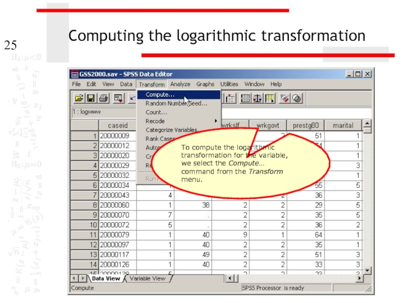
- 24. Problem 2 In the dataset GSS2000.sav, is
- 25. Computing the logarithmic transformation To compute the
- 26. Specifying the variable name and function First,
- 27. Adding the variable name to the function
- 28. Preventing illegal logarithmic values To solve this
- 29. The transformed variable The transformed variable which
- 30. The boxplot In this boxplot, the spread
- 31. The homogeneity of variance test The null
- 32. Homogeneity of variance test from the script
- 33. Other problems on homoscedasticity assumption A problem
- 34. Steps in answering questions about the assumption
- 35. Steps in answering questions about the assumption
Слайд 1Assumption of Homoscedasticity
Homoscedasticity
(also referred to as homogeneity of variance)
(also referred to
Transformations
Assumption of normality script
Practice problems
Слайд 2Assumption of Homoscedasticity
Homoscedasticity refers to the assumption that that the dependent
While it applies to independent variables at all three measurement levels, the methods that we will use to evaluation homoscedasticity requires that the independent variable be non-metric (nominal or ordinal) and the dependent variable be metric (ordinal or interval). When both variables are metric, the assumption is evaluated as part of the residual analysis in multiple regression.
Слайд 3Evaluating homoscedasticity
Homoscedasticity is evaluated for pairs of variables.
There are both
The graphical method is called a boxplot.
The statistical method is the Levene statistic which SPSS computes for the test of homogeneity of variances.
Neither of the methods is absolutely definitive.
Слайд 4Transformations
When the assumption of homoscedasticity is not supported, we can transform
We use the sample three common transformations that we used for normality: the logarithmic transformation, the square root transformation, and the inverse transformation.
All of these change the measuring scale on the horizontal axis of a histogram to produce a transformed variable that is mathematically equivalent to the original variable.
Слайд 5When transformations do not work
When none of the transformations results in
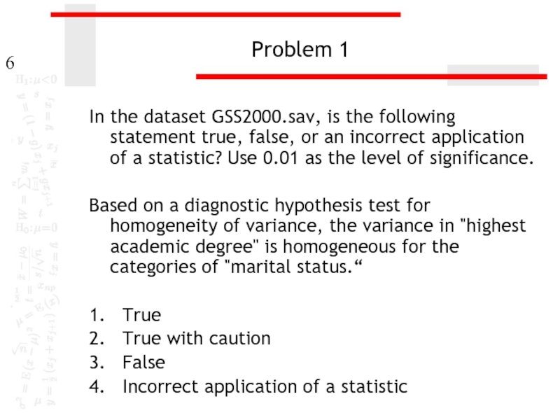
Слайд 6Problem 1
In the dataset GSS2000.sav, is the following statement true, false,
Based on a diagnostic hypothesis test for homogeneity of variance, the variance in "highest academic degree" is homogeneous for the categories of "marital status.“
1. True
2. True with caution
3. False
4. Incorrect application of a statistic
Слайд 7Request a boxplot
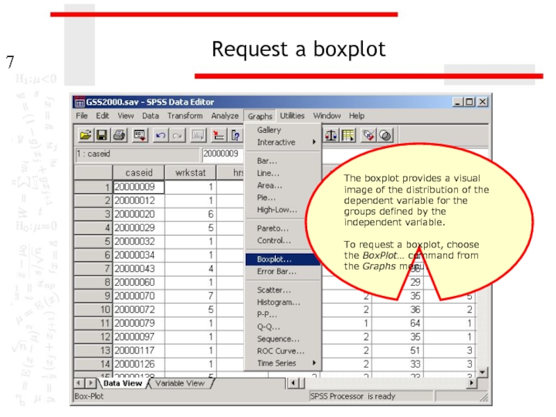
The boxplot provides a visual image of the distribution
To request a boxplot, choose the BoxPlot… command from the Graphs menu.
Слайд 8Specify the type of boxplot
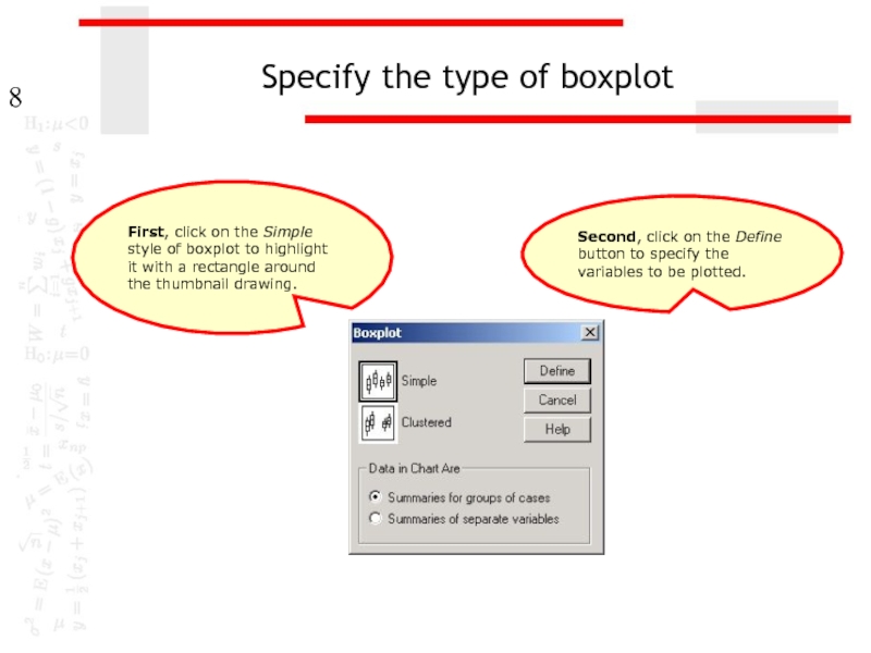
First, click on the Simple style of
Second, click on the Define button to specify the variables to be plotted.
Слайд 9Specify the dependent variable
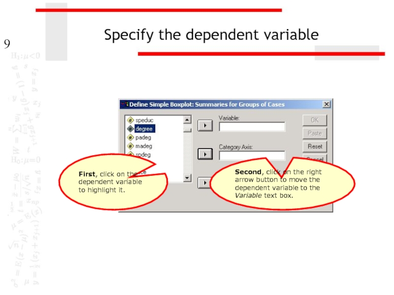
First, click on the dependent variable to highlight
Second, click on the right arrow button to move the dependent variable to the Variable text box.
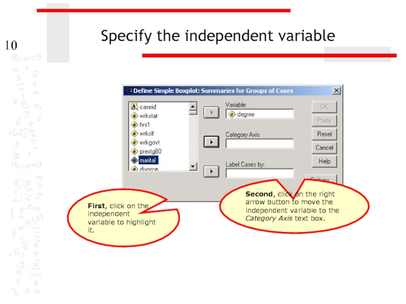
Слайд 10Specify the independent variable
First, click on the independent variable to highlight
Second, click on the right arrow button to move the independent variable to the Category Axis text box.
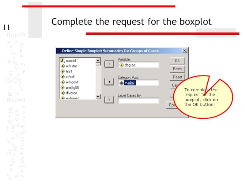
Слайд 11Complete the request for the boxplot
To complete the request for the
Слайд 12The boxplot
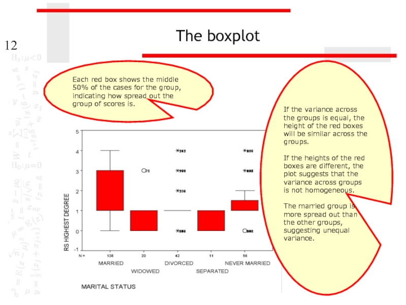
Each red box shows the middle 50% of the cases
If the variance across the groups is equal, the height of the red boxes will be similar across the groups.
If the heights of the red boxes are different, the plot suggests that the variance across groups is not homogeneous.
The married group is more spread out than the other groups, suggesting unequal variance.
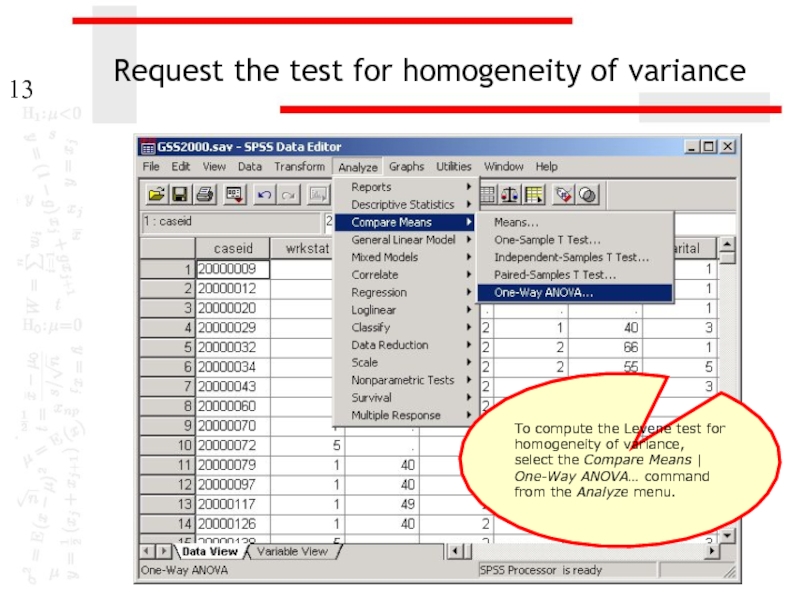
Слайд 13Request the test for homogeneity of variance
To compute the Levene test
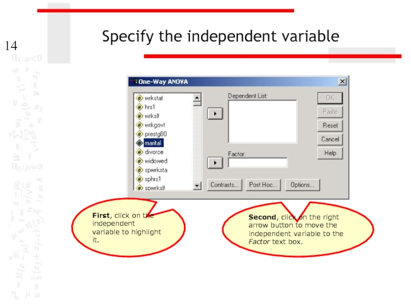
Слайд 14Specify the independent variable
First, click on the independent variable to highlight
Second, click on the right arrow button to move the independent variable to the Factor text box.
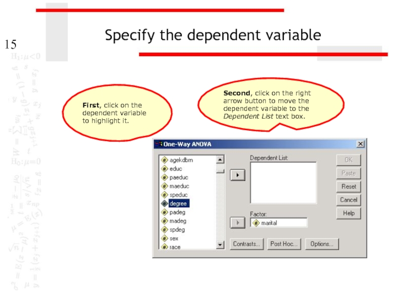
Слайд 15Specify the dependent variable
First, click on the dependent variable to highlight
Second, click on the right arrow button to move the dependent variable to the Dependent List text box.
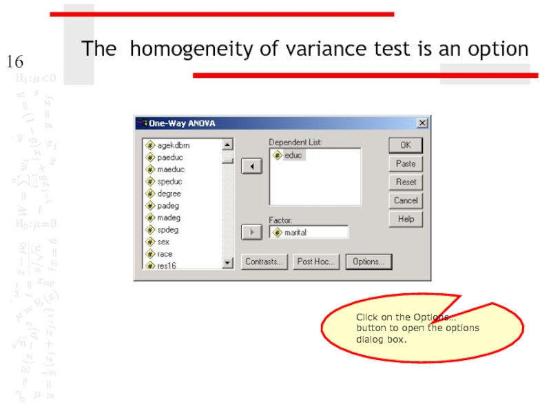
Слайд 16The homogeneity of variance test is an option
Click on the Options…
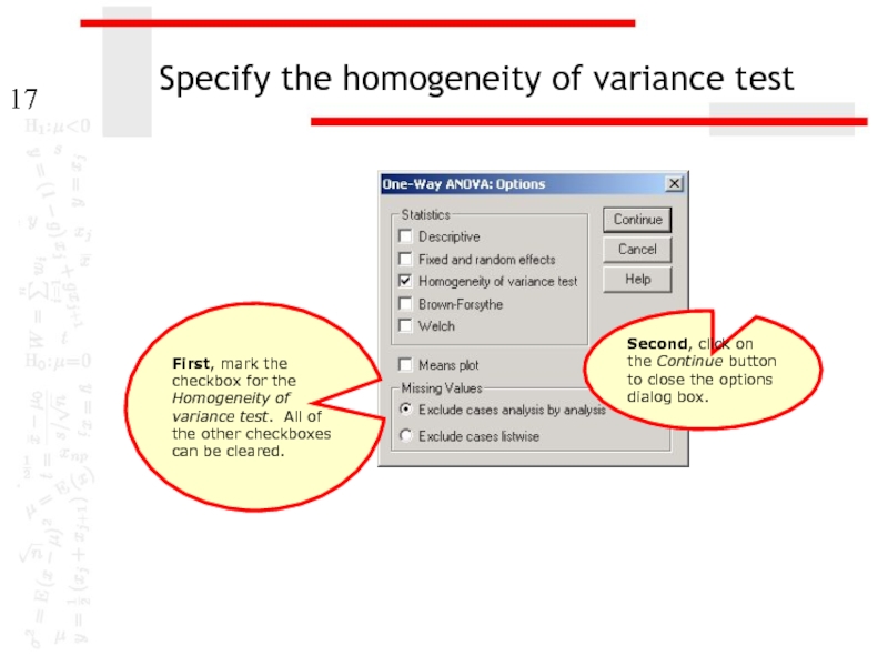
Слайд 17Specify the homogeneity of variance test
First, mark the checkbox for the
Second, click on the Continue button to close the options dialog box.
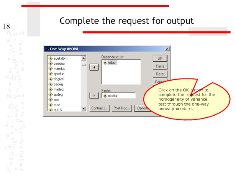
Слайд 18Complete the request for output
Click on the OK button to complete
Слайд 19Interpreting the homogeneity of variance test
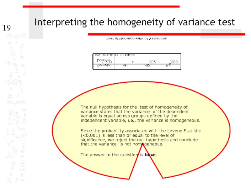
The null hypothesis for the test
Since the probability associated with the Levene Statistic (<0.001) is less than or equal to the level of significance, we reject the null hypothesis and conclude that the variance is not homogeneous.
The answer to the question is false.
Слайд 20The assumption of homoscedasticity script
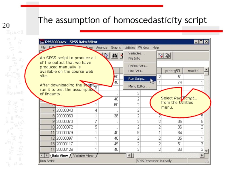
An SPSS script to produce all of
After downloading the script, run it to test the assumption of linearity.
Select Run Script… from the Utilities menu.
Слайд 21Selecting the assumption of homoscedasticity script
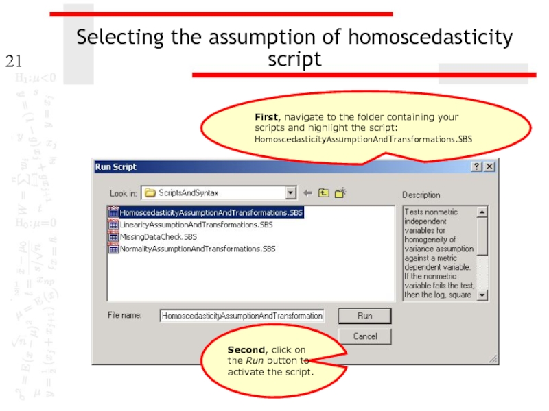
First, navigate to the folder containing
Second, click on the Run button to activate the script.
Слайд 22Specifications for homoscedasticity script
The default output is to do all of
Third, click on the OK button to run the script.
First, move the dependent variable to the Dependent (Y) Variable text box.
Second, move the independent variable to the Independent (X) Variables text box.
Слайд 23The test of homogeneity of variance
The script produces the same output
Слайд 24Problem 2
In the dataset GSS2000.sav, is the following statement true, false,
Based on a diagnostic hypothesis test for homogeneity of variance, the variance in "highest academic degree" is not homogeneous for the categories of "marital status." However, the variance in the logarithmic transformation of "highest academic degree" is homogeneous for the categories of "marital status."
1. True
2. True with caution
3. False
4. Incorrect application of a statistic
Слайд 25Computing the logarithmic transformation
To compute the logarithmic transformation for the variable,
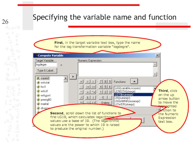
Слайд 26Specifying the variable name and function
First, in the target variable text
Second, scroll down the list of functions to find LG10, which calculates logarithmic values use a base of 10. (The logarithmic values are the power to which 10 is raised to produce the original number.)
Third, click on the up arrow button to move the highlighted function to the Numeric Expression text box.
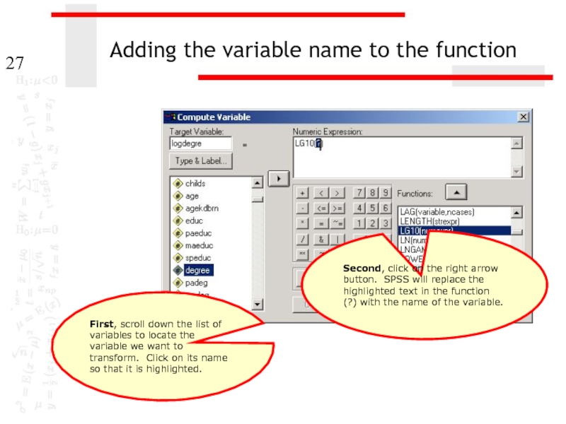
Слайд 27Adding the variable name to the function
First, scroll down the list
Second, click on the right arrow button. SPSS will replace the highlighted text in the function (?) with the name of the variable.
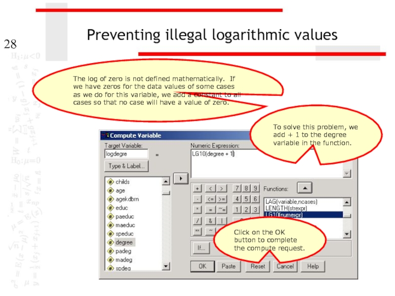
Слайд 28Preventing illegal logarithmic values
To solve this problem, we add + 1
The log of zero is not defined mathematically. If we have zeros for the data values of some cases as we do for this variable, we add a constant to all cases so that no case will have a value of zero.
Click on the OK button to complete the compute request.
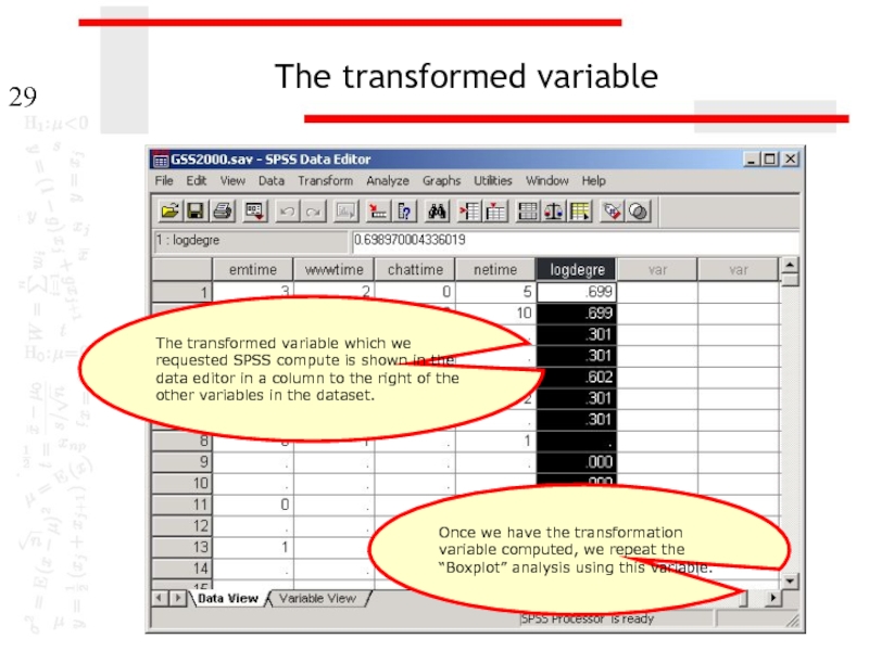
Слайд 29The transformed variable
The transformed variable which we requested SPSS compute is
Once we have the transformation variable computed, we repeat the “Boxplot” analysis using this variable.
Слайд 30The boxplot
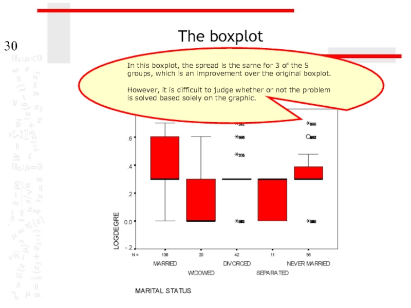
In this boxplot, the spread is the same for 3
However, it is difficult to judge whether or not the problem is solved based solely on the graphic.
Слайд 31The homogeneity of variance test
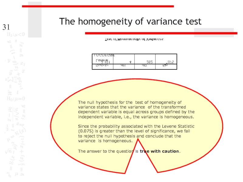
The null hypothesis for the test of
Since the probability associated with the Levene Statistic (0.075) is greater than the level of significance, we fail to reject the null hypothesis and conclude that the variance is homogeneous.
The answer to the question is true with caution.
Слайд 32Homogeneity of variance test from the script
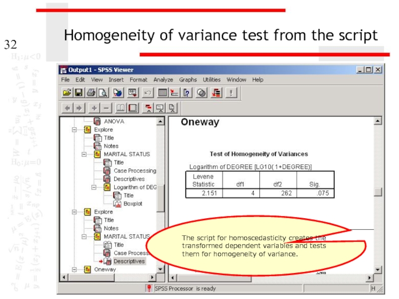
The script for homoscedasticity creates
Слайд 33Other problems on homoscedasticity assumption
A problem may ask about the assumption
A problem may ask about the assumption of homoscedasticity for an ordinal level dependent variable. If the variable or transformed variable satisfies the assumption of homogeneity of variance, the correct answer to the question is “True with caution” since we may be required to defend treating ordinal variables as metric.
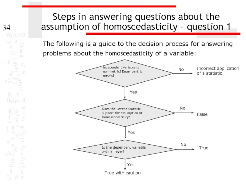
Слайд 34Steps in answering questions about the assumption of homoscedasticity – question
The following is a guide to the decision process for answering
problems about the homoscedasticity of a variable:
Does the Levene statistic support the assumption of homoscedasticity?
False
Is the dependent variable ordinal level?
True
True with caution
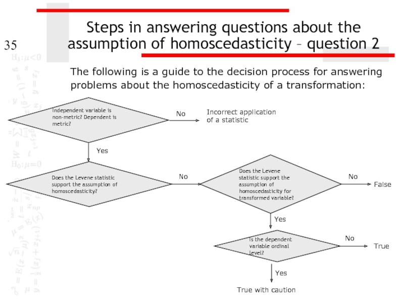
Слайд 35Steps in answering questions about the assumption of homoscedasticity – question
The following is a guide to the decision process for answering
problems about the homoscedasticity of a transformation:
Does the Levene statistic support the assumption of homoscedasticity?
Does the Levene statistic support the assumption of homoscedasticity for transformed variable?
Is the dependent variable ordinal level?
False
True
True with caution

