of Mechanical Engineering,
School of Engineering,
Nazarbayev University
- Главная
- Разное
- Дизайн
- Бизнес и предпринимательство
- Аналитика
- Образование
- Развлечения
- Красота и здоровье
- Финансы
- Государство
- Путешествия
- Спорт
- Недвижимость
- Армия
- Графика
- Культурология
- Еда и кулинария
- Лингвистика
- Английский язык
- Астрономия
- Алгебра
- Биология
- География
- Детские презентации
- Информатика
- История
- Литература
- Маркетинг
- Математика
- Медицина
- Менеджмент
- Музыка
- МХК
- Немецкий язык
- ОБЖ
- Обществознание
- Окружающий мир
- Педагогика
- Русский язык
- Технология
- Физика
- Философия
- Химия
- Шаблоны, картинки для презентаций
- Экология
- Экономика
- Юриспруденция
Control systems презентация
Содержание
- 1. Control systems
- 2. By failing to prepare, you are preparing to fail. Benjamin Franklin
- 3. Contents -Review of Previous Lectures -System Response Analysis
- 4. Review Once transfer function is obtained, we
- 5. Review-Block Diagram Three Elementary Block Diagrams Series connection Parallel connection Negative Feedback connection
- 6. Negative feedback :Single-loop gain The gain of
- 7. Review-Block Diagram
- 8. Table 2.6 (continued) Block Diagram Transformations Review-Block Diagram
- 9. Review-Block Diagram Practice: Find the transfer function of the following block diagram
- 10. Review-Block Diagram Practice:
- 11. Review-Block Diagram
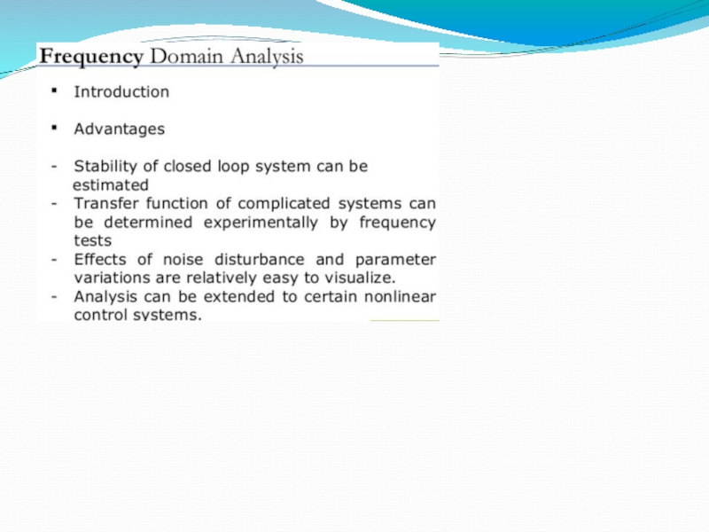
- 12. Time domain and frequency domain
- 17. Poles and Zeros K is the transfer
- 18. System Response: Complex system
- 19. System Response: Stability in s-plane
- 20. Key points: Effect of Poles and Zeros
- 21. Example: Consider the following transfer function
- 22. System Response: Effect of pole location
- 23. Example: Consider the following transfer function
- 24. Time-Domain Specification To measure the performance of
- 25. Time-Domain Specification Test Input Signals step input
- 26. Time-Domain Specification Example The transfer function: The system response to a unit step input (A=1):
- 27. System Response Example 2: Consider the
- 28. First Order System Response
- 29. Example 1: Consider the following transfer function
- 30. First Order System Response- Impulse response
- 31. Let us consider the following closed-loop system:
- 32. Standard Second Order System
- 33. Figure 3.24 Graphs of regions in
- 34. Transformation of the specification to the s-plane
- 35. Mp? Standard Second Order System
- 36. Poles (roots) location of the second order
- 37. Classification of Type Response of 2nd Order Systems Undamped: ζ=0 Under-damped: 0
- 38. As ζ decreases, the response becomes increasingly oscillatory. Standard Second Order System
- 39. Time-Domain Specification Standard performance measures are usually
- 40. Time-Domain Specification Standard performance measures are usually
- 41. Time-Domain Specification -Rise Time, Tr- A precise
- 42. Time-Domain Specification Maximum overshoot (in percentage) is defined as -Maximum Overshoot, Mp
- 43. Time-Domain Specification Tp is found by differentiating
- 44. Time-Domain Specification -Settling Time Ts-
- 45. Time-Domain Specification Exercise # 1 Find
- 46. Time-Domain Specification Exercise # 2 Find
- 47. Exercise # 3 If the system response
- 48. Exercise # 4 Problem# If the system
- 49. Time-Domain Specification Exercise # 5 Find
- 50. Time-Domain Specification Exercise # 6 Find
- 51. Time-Domain Specification Exercise # 7 Find
- 52. Figure - Multiple-loop feedback control system.
- 53. Figure 2.27 Block diagram reduction of
- 54. System Response Consider the following transfer function
- 55. Impulse response Answer
- 56. Midterm Exam March 4, 2016, Friday, Time:8.00-9.00 Venue-6.141 & 5.103 Topics- Cover Until February
- 58. Tell me, I will forget! Show
- 59. Further Reading Franklin, et. al., Chapter 3
Слайд 1
Control Systems
Dynamic Response: Dynamic Response Analysis, Steady State Error
Md Hazrat Ali
Department


Слайд 4Review
Once transfer function is obtained, we can start to analyze the
response of the system it represents .
A block diagram is a convenient tool to visualize the systems as a collection of interrelated subsystems that emphasize the relationships among the system variables.
Signal flow graph and Mason’s gain formula are used to determine the transfer function of the complex block diagram.
A block diagram is a convenient tool to visualize the systems as a collection of interrelated subsystems that emphasize the relationships among the system variables.
Signal flow graph and Mason’s gain formula are used to determine the transfer function of the complex block diagram.

Слайд 5Review-Block Diagram
Three Elementary Block Diagrams
Series connection
Parallel connection
Negative Feedback connection

Слайд 6Negative feedback :Single-loop gain
The gain of a single-loop negative feedback system
is given by the forward gain divided by the sum of 1 plus the loop gain.
Franklin et.al- pp.122
Franklin et.al- pp.122


 Block Diagram TransformationsReview-Block Diagram")


Слайд 17Poles and Zeros
K is the transfer gain
The roots of numerator is
called zeros of the system. Zeros correspond to signal transmission-blocking properties.
The roots of denominator are called poles of the system. Poles determine the stability properties and natural or unforced behavior of the system.
Poles and zeros can be complex quantities.
zi=pi, cancellation of pole-zero may lead to undesirable system properties.
The roots of denominator are called poles of the system. Poles determine the stability properties and natural or unforced behavior of the system.
Poles and zeros can be complex quantities.
zi=pi, cancellation of pole-zero may lead to undesirable system properties.


Слайд 21Example:
Consider the following transfer function
Determine:
Poles and Zeros?
System Response


Слайд 23Example:
Consider the following transfer function
Determine:
Poles and Zeros?
System Response

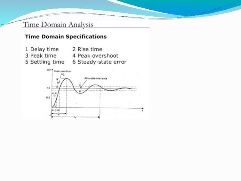
Слайд 24Time-Domain Specification
To measure the performance of a system we use standard
test input signals. This allows us to compare the performance of our system for different designs.
The standard test inputs used are the step input, the ramp input, and the parabolic input.
A unit impulse function is also useful for test signal purpose.
The standard test inputs used are the step input, the ramp input, and the parabolic input.
A unit impulse function is also useful for test signal purpose.
Test Input Signals

Слайд 25Time-Domain Specification
Test Input Signals
step input
ramp input
parabolic input
The step input is the
easiest to generate and evaluate and is usually chosen for performance tests.

Слайд 26Time-Domain Specification
Example
The transfer function:
The system response to a unit step input
(A=1):
:")
Слайд 27System Response
Example 2:
Consider the following transfer function
Determine:
impulse response


Слайд 29Example 1:
Consider the following transfer function
Determine:
impulse response(response when r(t)
is
impulse function)
Classify stability
impulse function)
Classify stability
First Order System Response
 is impulse function)Classify stability")

Слайд 31Let us consider the following closed-loop system:
The TF of the closed-loop
system:
Utilizing the general notation of 2nd Order System:
Where ωn is natural frequency and ζ is damping ratio
Utilizing the general notation of 2nd Order System:
Where ωn is natural frequency and ζ is damping ratio
Standard Second Order System


Слайд 33Figure 3.24 Graphs of regions in the s-plane delineated by
certain transient requirements: (a) rise time; (b) overshoot;
(c) settling time; (d) composite of all three requirements
Transformation of the specification to the s-plane
 rise")
Слайд 34Transformation of the specification to the s-plane
Example 3.25
Find allowable regions in
the s-plane for the poles transfer function of system if the system response requirements are tr ≤ 0.6, Mp <= 10% and ts <= 3 sec.


Слайд 36Poles (roots) location of the second order complex system.
Standard Second Order
System
Standard Second Order System
 location of the second order complex system.Standard Second Order SystemStandard Second Order System")
Слайд 37Classification of Type Response of 2nd Order Systems
Undamped: ζ=0
Under-damped: 0
ζ=1
Over-damped: ζ>1
Standard Second Order System


Слайд 39Time-Domain Specification
Standard performance measures are usually defined in term of the
step response of a 2nd order systems:

Слайд 40Time-Domain Specification
Standard performance measures are usually defined in term of the
step response of a 2nd order systems:
Rise time, Tr : time needed from 0 to 100% of fv for underdamped systems and Tr1 from 10-90% of fv for overdamped systems.
The settling time ts is the time it takes the system transient to decay.
The overshoot Mp is the maximum amount of the system overshoots its final value divided by its final value.
The peak time tp, is the time it takes the system to reach the maximum overshoot.

Слайд 41Time-Domain Specification
-Rise Time, Tr-
A precise analytical relationship between rise time and
damping ratio ζ cannot be found. However, it can be found using numerically using computer.
A rough estimation of the rise time is as follows

Слайд 42Time-Domain Specification
Maximum overshoot (in percentage) is defined as
-Maximum Overshoot, Mp
 is defined as-Maximum Overshoot, Mp")
Слайд 43Time-Domain Specification
Tp is found by differentiating y(t) and finding the first
zero crossing after t=0.
-Peak Time Tp-
 and finding the first zero crossing after t=0.-Peak")
Слайд 44Time-Domain Specification
-Settling Time Ts-
For a second order system, we seek to
determine the time Ts for which the response remains within certain percentage (1%, 2% ) of the final value.
For 1% settling time
For 2% settling time

Слайд 45Time-Domain Specification
Exercise # 1
Find Tr, Tp, Mp and Ts for the
following transfer function:

Слайд 46Time-Domain Specification
Exercise # 2
Find Tr, Tp, Mp and Ts for the
following transfer function:


Слайд 48Exercise # 4
Problem# If the system response requirements are tr =
0.6, Mp = 10% and ts = 3 sec.
Find:
For 1% settling time

Слайд 49Time-Domain Specification
Exercise # 5
Find Tr, Tp, Mp and Ts for the
following transfer function:

Слайд 50Time-Domain Specification
Exercise # 6
Find Tr, Tp, Mp and Ts for the
following transfer function:

Слайд 51Time-Domain Specification
Exercise # 7
Find Tr, Tp, Mp and Ts for the
following transfer function:

Слайд 52Figure - Multiple-loop feedback control system.
Example - Block diagram
Find
TF from the given block diagram


Слайд 54System Response
Consider the following transfer function
Determine:
i) Impulse response graphically
ii)
Classify stability
Find TF from the given block diagram
 Impulse response graphically ii) Classify stability Find TF")

Слайд 56Midterm Exam
March 4, 2016, Friday, Time:8.00-9.00
Venue-6.141 & 5.103
Topics- Cover Until February

Слайд 58Tell me, I will forget! Show me, I may remember! Involve me, I
will understand!
Benjamin Franklin

Слайд 59Further Reading
Franklin, et. al., Chapter 3
Section 3.1-3.6
Richard C. Dorf et.al, Chapter
3
Additional notes are uploaded on moodle
Additional notes are uploaded on moodle