- Главная
- Разное
- Дизайн
- Бизнес и предпринимательство
- Аналитика
- Образование
- Развлечения
- Красота и здоровье
- Финансы
- Государство
- Путешествия
- Спорт
- Недвижимость
- Армия
- Графика
- Культурология
- Еда и кулинария
- Лингвистика
- Английский язык
- Астрономия
- Алгебра
- Биология
- География
- Детские презентации
- Информатика
- История
- Литература
- Маркетинг
- Математика
- Медицина
- Менеджмент
- Музыка
- МХК
- Немецкий язык
- ОБЖ
- Обществознание
- Окружающий мир
- Педагогика
- Русский язык
- Технология
- Физика
- Философия
- Химия
- Шаблоны, картинки для презентаций
- Экология
- Экономика
- Юриспруденция
Mathematics in Finance презентация
Содержание
- 1. Mathematics in Finance
- 2. Contents American options The obstacle problem Discretisation methods Matlab results Recent insights and developments
- 3. 1. American options American options can
- 4. Bounds for prices (no dividends) For American options: For European options: Reminder: put-call parity
- 5. Why is
- 6. What about put options? For put options,
- 7. American options are more expensive than European options Comparison European-American options
- 8. An optimum time for exercising…. (1) Statement:
- 9. An optimum time for exercising…. (2) The
- 10. Derivation of equation and BC’s (1) For
- 11. Derivation of equation and BC’s (2) As
- 12. Summary of equation and BC’s The value
- 13. How to solve? Free boundary problems can
- 14. 2. The obstacle problem Consider a rope:
- 16. The linear complimentarity problem We rewrite the
- 17. Formulation without second derivatives Lemma 1: Define
- 18. What about minimum length? The latter is
- 19. Summarizing so far The obstacle problem can
- 20. 3. Discretisation methods
- 21. Finite difference method (1) If we choose
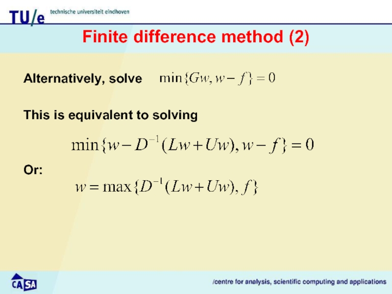
- 22. Finite difference method (2) Alternatively, solve
- 23. Finite difference method (3) We can use
- 24. Finite element method (1) As the basis
- 25. Finite element method (2) These expressions can
- 26. Summary: comparison of FD and FEM Finite
- 27. 4. Implementation in Matlab
- 28. Back to American options The problem for
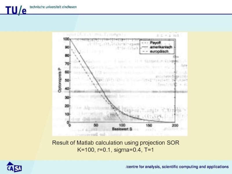
- 29. Result of Matlab calculation using projection SOR K=100, r=0.1, sigma=0.4, T=1
- 30. Number of iterations in projection SOR method Depending on the overrelaxation parameter omega
- 31. 5. Recent insights and developments
- 32. Historical account First widely-used methods using FD
- 33. Recent work (1) Some people concentrate on
- 34. Recent work (2) In S. Berridge
Слайд 1Mathematics in Finance
Numerical solution of free boundary problems: pricing of American
Wil Schilders (June 2, 2005)
Слайд 2Contents
American options
The obstacle problem
Discretisation methods
Matlab results
Recent insights and developments
Слайд 31. American options
American options can be executed any time before
We will derive a partial differential inequality from which a fair price for an American option can be calculated.
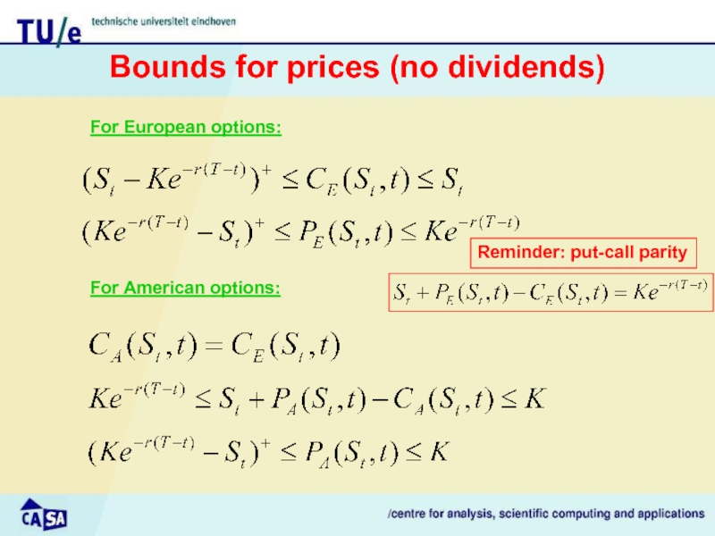
Слайд 4Bounds for prices (no dividends)
For American options:
For European options:
Reminder: put-call parity
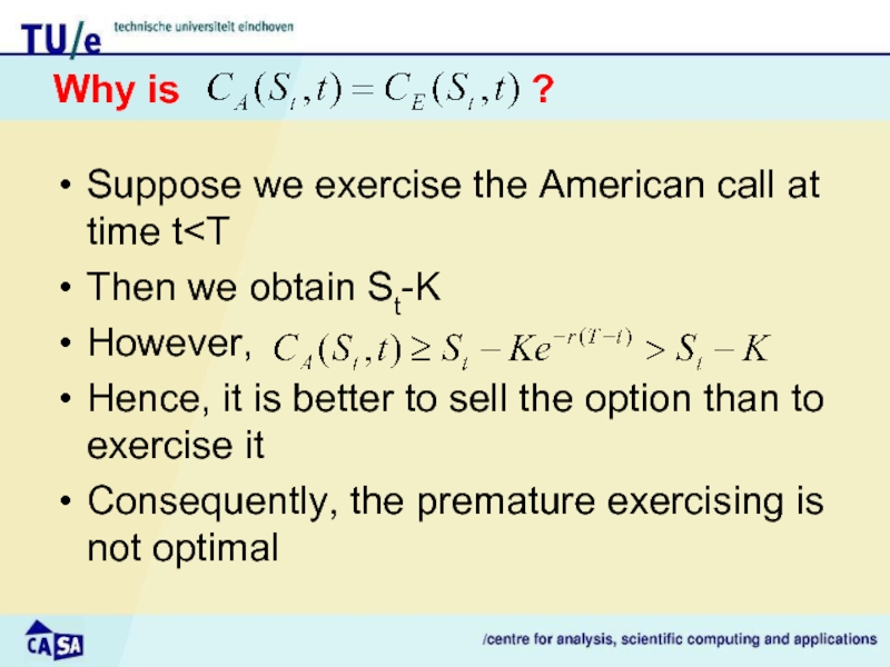
Слайд 5Why is
Suppose we exercise the American call at time t
However,
Hence, it is better to sell the option than to exercise it
Consequently, the premature exercising is not optimal
Слайд 6What about put options?
For put options, a similar reasoning shows that
Слайд 7American options are more expensive
than European options
Comparison European-American options
Слайд 8An optimum time for exercising…. (1)
Statement: There is Sf such that
Proof: Let be a portfolio. As soon as
, the option can be exercised since we can invest the amount
at interest rate r. For it is not worthwhile, since the value of the portfolio before exercising is ,
but after exercising is equal to .
Слайд 9An optimum time for exercising…. (2)
The value Sf depends on time,
This free boundary value is unknown, and must be determined in addition to the option price! Therefore, we have a free boundary value problem that must be solved.
Слайд 10Derivation of equation and BC’s (1)
For S up to Sf the
For larger S, the put option satisfies the Black-Scholes equation since, in this case, we keep the option which can then be valued as a European option
For S>>K, value is negligible:
Also, we must have:
Not sufficient, since we must also find Sf
Слайд 11Derivation of equation and BC’s (2)
As extra condition, we require that
is continuous at S=Sf(t). Since, for S
this can also be written in the form:
Слайд 12Summary of equation and BC’s
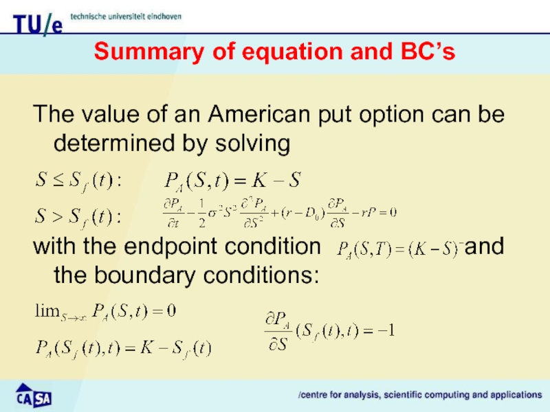
The value of an American put option
with the endpoint condition and the boundary conditions:
Слайд 13How to solve?
Free boundary problems can be rewritten in the form
These can be solved by numerical methods
To illustrate the alternatives and the numerical solution techniques, we will give an example
Слайд 142. The obstacle problem
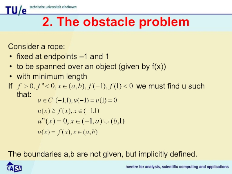
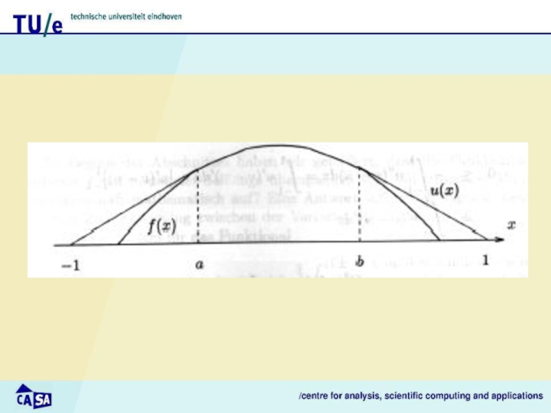
Consider a rope:
fixed at endpoints –1 and 1
to
with minimum length
If we must find u such that:
The boundaries a,b are not given, but implicitly defined.
Слайд 16The linear complimentarity problem
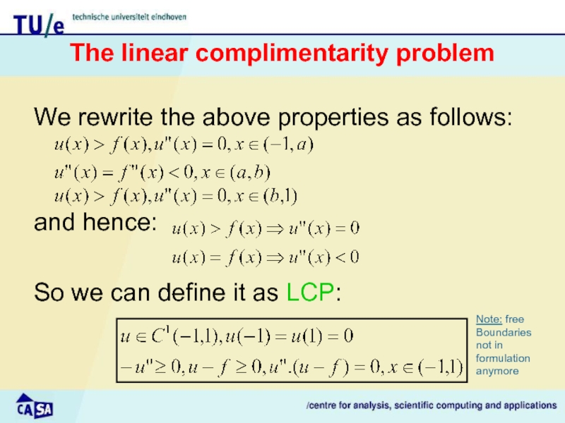
We rewrite the above properties as follows:
and hence:
So
Note: free
Boundaries not in formulation anymore
Слайд 17Formulation without second derivatives
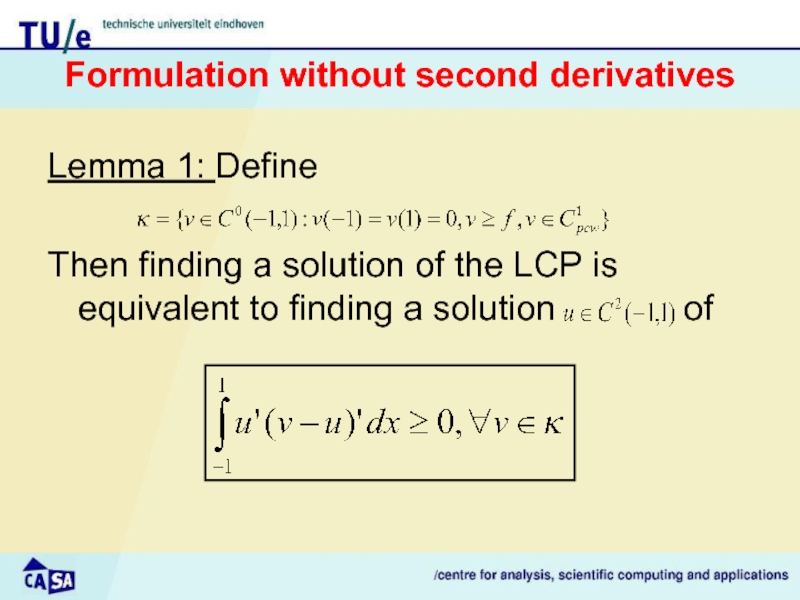
Lemma 1: Define
Then finding a solution of the
Слайд 18What about minimum length?
The latter is again equal to the following
Find with the property
where
Слайд 19Summarizing so far
The obstacle problem can be formulated
As a free boundary
As a linear complimentarity problem
As a variational inequality
As a minimization problem
We will now see how the obstacle problem can be solved numerically.
Слайд 21Finite difference method (1)
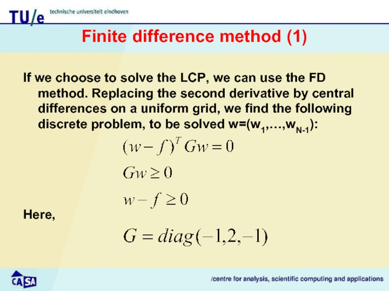
If we choose to solve the LCP, we
Here,
Слайд 23Finite difference method (3)
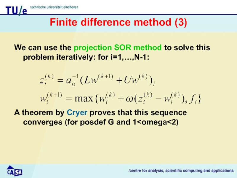
We can use the projection SOR method to
A theorem by Cryer proves that this sequence converges (for posdef G and 1
Слайд 24Finite element method (1)
As the basis we use the variational inequality
The
Hence, we may write
Слайд 25Finite element method (2)
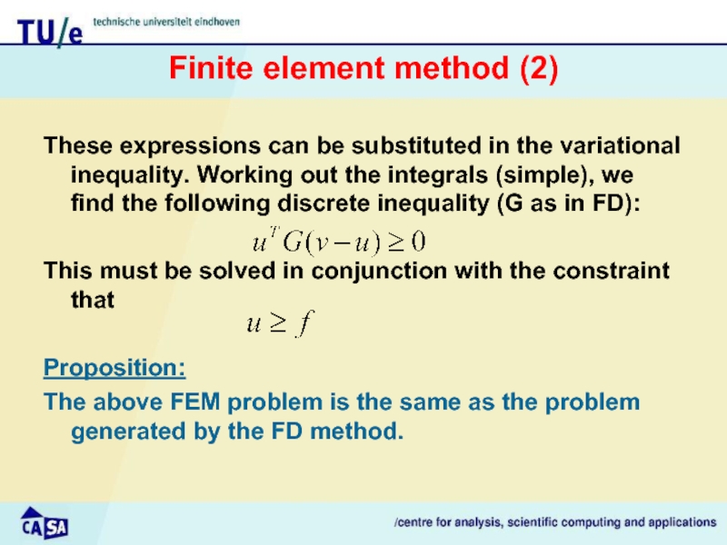
These expressions can be substituted in the variational
This must be solved in conjunction with the constraint that
Proposition:
The above FEM problem is the same as the problem generated by the FD method.
Слайд 28Back to American options
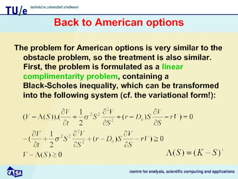
The problem for American options is very similar
Слайд 30Number of iterations in projection SOR method
Depending on the overrelaxation parameter
Слайд 32Historical account
First widely-used methods using FD by Brennan and Schwartz (1977)
Wilmott, Dewynne and Howison (1993) introduced implicit FD methods for solving PDE’s, by solving an LCP at each step using the projected SOR method of Cryer (1971)
Huang and Pang (1998) gave a nice survey of state-of-the-art numerical methods for solving LCP’s. Unfortunately, they assume a regular FD grid
Слайд 33Recent work (1)
Some people concentrate on Monte Carlo methods to evaluate
More popular are the QMC methods that are more efficient (Niederreiter, 1992)
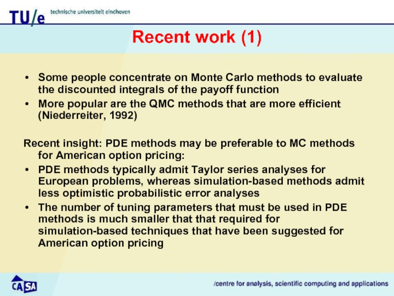
Recent insight: PDE methods may be preferable to MC methods for American option pricing:
PDE methods typically admit Taylor series analyses for European problems, whereas simulation-based methods admit less optimistic probabilistic error analyses
The number of tuning parameters that must be used in PDE methods is much smaller that that required for simulation-based techniques that have been suggested for American option pricing
Слайд 34Recent work (2)
In
S. Berridge
“Irregular Grid Methods for Pricing High-Dimensional American Options”
(Tilburg
an account is given of several methods based on the use of irregular grids.
