- Главная
- Разное
- Дизайн
- Бизнес и предпринимательство
- Аналитика
- Образование
- Развлечения
- Красота и здоровье
- Финансы
- Государство
- Путешествия
- Спорт
- Недвижимость
- Армия
- Графика
- Культурология
- Еда и кулинария
- Лингвистика
- Английский язык
- Астрономия
- Алгебра
- Биология
- География
- Детские презентации
- Информатика
- История
- Литература
- Маркетинг
- Математика
- Медицина
- Менеджмент
- Музыка
- МХК
- Немецкий язык
- ОБЖ
- Обществознание
- Окружающий мир
- Педагогика
- Русский язык
- Технология
- Физика
- Философия
- Химия
- Шаблоны, картинки для презентаций
- Экология
- Экономика
- Юриспруденция
Unemployment rate презентация
Содержание
- 1. Unemployment rate
- 2. Let’s review our voyage to date: We
- 3. What picture do you have in mind
- 4. Understanding business cycles Major elements of
- 5. Output gap and recessions
- 6. Unemployment and recessions
- 7. Unemployment and vacancies (2000-2010)
- 8. So what’s the big problem for economics?
- 10. This has been the approach up to now.
- 11. We now move to a different set of assumptions/observations
- 12. Major approaches to business cycles Classical: market
- 13. Real output (Y) Expenditures C+I+G+NX Y* E*
- 14. Real output (Y) Price (P) AD AS
- 15. IS-LM model The major tool for showing
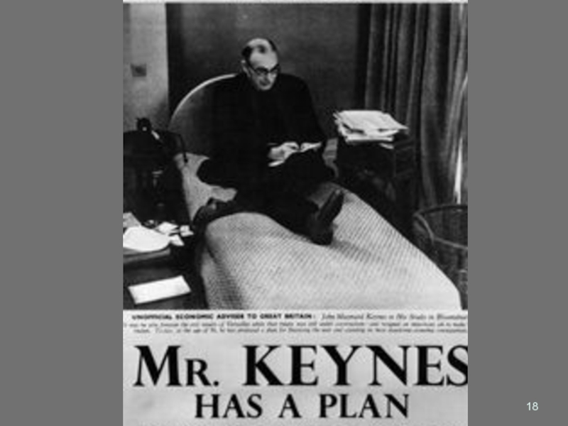
- 16. The Founder of Macroeconomics Gwendolen Darwin Raverat
- 17. Keynes on Why macroeconomics is difficult or
- 19. Where are we? We are now attempting
- 20. IS curve (expenditures) Basic idea: describes equilibrium
- 21. which gives the IS curve:
- 22. LM curve (financial markets) The LM curve
- 23. Summary of IS-LM Y ≡
- 24. Overall Macroeconomic Equilibrium We now are
- 25. Real output (Y) interest rate (r) IS(r;
- 26. SOME BASICS OF THE IS-LM MODEL
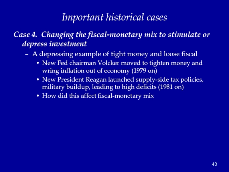
- 27. Now several interesting cases Case 1. A
- 28. Real output (Y) interest rate (r) IS
- 29. More on financial issues… Case 1A. A
- 30. Case 2. What are the effects of
- 31. Real output (Y) interest rate (r) IS
- 32. Real output (Y) interest rate (r) IS
- 33. Multiplier Estimates by the CBO Congressional Budget Office, Estimated Impact of the ARRA, April 2010

Слайд 2Let’s review our voyage to date:
We have analyzed:
Measuring economic activity
Aggregate production
functions and distribution
Classical AS and AD (flexible w and p)
Financial macro (including money)
Open-economy macro
We now move on to
Business cycles, Keynesian economics, and the IS-LM model
Classical AS and AD (flexible w and p)
Financial macro (including money)
Open-economy macro
We now move on to
Business cycles, Keynesian economics, and the IS-LM model

Слайд 3What picture do you have in mind when you think of
business cycles?
“Note that the pattern of cycles is irregular. No two business cycles are quite the same. No exact formula, such as might apply to the revolutions of the planets or of a pendulum, can be used to predict the duration and timing of business cycles. Rather, in their irregularities, business cycles more closely resemble the fluctuations of the weather.” (Paul Samuelson)
“Note that the pattern of cycles is irregular. No two business cycles are quite the same. No exact formula, such as might apply to the revolutions of the planets or of a pendulum, can be used to predict the duration and timing of business cycles. Rather, in their irregularities, business cycles more closely resemble the fluctuations of the weather.” (Paul Samuelson)

Слайд 4Understanding business cycles
Major elements of cycles
short-period (1-3 yr) erratic fluctuations in
output
pro-cyclical movements of employment, profits, prices
counter-cyclical movements in unemployment
appearance of “involuntary” unemployment in recessions
Historical trends
lower volatility of output, inflation over time (until 2008)
movement from stable prices to rising prices since WW II
pro-cyclical movements of employment, profits, prices
counter-cyclical movements in unemployment
appearance of “involuntary” unemployment in recessions
Historical trends
lower volatility of output, inflation over time (until 2008)
movement from stable prices to rising prices since WW II
 erratic fluctuations in outputpro-cyclical movements of")


")
Слайд 8So what’s the big problem for economics?
Many economists worry that there
are no firm “microeconomic foundations” for Keynesian business cycle theory.
What should we do?
- throw out the theory?
- live with this inadequacy?
What should we do?
- throw out the theory?
- live with this inadequacy?


Слайд 12Major approaches to business cycles
Classical: market clearing: supply-side cycles with vertical
AS curve:
Real business cycles: major active classical species today
Keynesian and offshoots: non-market clearing with non-vertical AS
Essential to have non-classical AS
Fixed or sticky p and w
AD shifts affect output and employment
Underlying theory incompletely understook – active area of research
Basic models in Keynesian approach
“Keynesian cross” (Econ 116)
AS-AD (Econ 116)
IS-LM (Econ 122)
Mankiw’s dynamic model (later)
Open-economy in short run: Mundell-Fleming (later in course)

Слайд 13Real output (Y)
Expenditures
C+I+G+NX
Y*
E*
Equilibrium
output
Keynesian Cross Diagram:
Output where planned expenditure equals output
Output where planned expenditure equals output
ExpendituresC+I+G+NXY*E*Equilibrium output Keynesian Cross Diagram: Output where planned expenditure equals output")
Price (P)ADASY*P*ClassicalmodelFix-priceModel (IS-LM)AS-AD approachAD")
Слайд 15IS-LM model
The major tool for showing the impact of monetary and
fiscal polices, along with the effect of various shocks, in a short-run Keynesian situation.
Key assumptions
Fixed prices (P=1)
Unemployed resources (Y < potential Y = Mankiw’s natural Y)
Closed economy (not essential and will be considered later)
Key assumptions
Fixed prices (P=1)
Unemployed resources (Y < potential Y = Mankiw’s natural Y)
Closed economy (not essential and will be considered later)


Слайд 17Keynes on Why macroeconomics is difficult
or
Why the models are so confusing!
Professor
Planck, of Berlin, the famous originator of the Quantum Theory, once remarked to me that in early life he had thought of studying economics, but had found it too difficult! Professor Planck could easily master the whole corpus of mathematical economics in a few days. But the amalgam of logic and intuition and the wide knowledge of facts, most of which are not precise, which is required for economic interpretation in its highest form is, quite truly, overwhelmingly difficult.
(“Biography of Marshall,” Economic Journal, 1924)
(“Biography of Marshall,” Economic Journal, 1924)

Слайд 19Where are we?
We are now attempting to understand the basic features
of business cycles.
Aggregate supply (AS) in this model is real simple: a horizontal AS curve with p=1.
AD relies on the IS-LM model, which is a very simple two-market model of the determinants of AD.
The two markets are
- goods (IS)
- financial (LM)
Aggregate supply (AS) in this model is real simple: a horizontal AS curve with p=1.
AD relies on the IS-LM model, which is a very simple two-market model of the determinants of AD.
The two markets are
- goods (IS)
- financial (LM)

Слайд 20IS curve (expenditures)
Basic idea: describes equilibrium in goods market
Finds Y where
planned I = planned S or planned expenditure = planned output
Basic set of equations:
Y = C + I + G
C = a + b(Y-T)
T = T0 + τ Y [note assume income tax, τ = marginal tax rate]
I = I0 –dr [note i = r because fixed P]
G = G0
Basic set of equations:
Y = C + I + G
C = a + b(Y-T)
T = T0 + τ Y [note assume income tax, τ = marginal tax rate]
I = I0 –dr [note i = r because fixed P]
G = G0
Basic idea: describes equilibrium in goods marketFinds Y where planned I = planned")
Слайд 21which gives the IS curve:
Y =
a - bT0 + G0 + I0 - dr
1 - b(1- τ)
Y = μ [A0 - dr]
where
A0 = autonomous spending = a - bT0 + G0 + I0
μ = multiplier = 1/[(1 - b(1- τ)]
or in terms of solving for the interest rate: r = (A0 - Y/μ ) / d
which we graph as the IS curve.
1 - b(1- τ)
Y = μ [A0 - dr]
where
A0 = autonomous spending = a - bT0 + G0 + I0
μ = multiplier = 1/[(1 - b(1- τ)]
or in terms of solving for the interest rate: r = (A0 - Y/μ ) / d
which we graph as the IS curve.

Слайд 22LM curve (financial markets)
The LM curve represents equilibrium in financial markets,
or where the supply and demand for money are equilibrated.
Ms determined by the central bank Ms = M0
Standard interest-elastic demand for money:* Md = L(i, Y) = kY- hi
Equilibrium in the money market is Md = Ms
This leads to LM curve: i = ( kY - M0 )/h
Not the best way to understand financial markets;
will consider alternative approach later.
* Note that interest rate is nominal rate here to reflect the difference between the interest rate on bonds and that on money.
The LM curve represents equilibrium in financial markets, or where the supply")
Слайд 23Summary of IS-LM
Y ≡ C + I + G
C = a + b(Y-T)
T = T0 + τY
I = I0 – dr
G = G0
Ms = M0
Md = L(i, Y) = kY- hi = kY- hr [r = i because zero inflation]
All this yields
hμ dμ Y* = ―――――― A0 + ――――― M0
dμk + h dμk + h
where
A0 = autonomous spending = a - bT0 + G0 + I0
μ = expenditure multiplier at constant r = 1/[(1 - b(1- τ)]
T = T0 + τY
I = I0 – dr
G = G0
Ms = M0
Md = L(i, Y) = kY- hi = kY- hr [r = i because zero inflation]
All this yields
hμ dμ Y* = ―――――― A0 + ――――― M0
dμk + h dμk + h
where
A0 = autonomous spending = a - bT0 + G0 + I0
μ = expenditure multiplier at constant r = 1/[(1 - b(1- τ)]
")
Слайд 24Overall Macroeconomic Equilibrium
We now are looking for equilibrium of both markets.
That is, when both goods market and money market are in equilibrium.
Closed economy and zero inflation (so i=r)
This is the solution or intersection of IS and LM.
hμ dμ Y* = ―――――― A0 + ――――― M0
dμk + h dμk + h
Impact of fiscal and monetary policy function of the different parameters. Easiest to understand using the IS-LM diagram.
Closed economy and zero inflation (so i=r)
This is the solution or intersection of IS and LM.
hμ dμ Y* = ―――――― A0 + ――――― M0
dμk + h dμk + h
Impact of fiscal and monetary policy function of the different parameters. Easiest to understand using the IS-LM diagram.

interestrate(r)IS(r; G, T0 ,τ …)LM(r; M, risk premium,…)Y*r*IS-LM diagram")
Слайд 26 SOME BASICS OF THE IS-LM MODEL
Have two major kinds of
shocks in business cycles:
IS: investment, consumption, foreign trade, …
LM: financial markets, monetary policy, exchange rates,…
Because of monetary reaction, expenditure multiplier is almost surely less than standard Keynesian multiplier due to crowding out.
Proof: IS-LM multiplier = μ/[dμk/h + 1] < μ = simplest multiplier
Can usually diagnose shock by the relative movements of output and interest rates (compare Vietnam War and 1979-82 on next slide)

Слайд 27Now several interesting cases
Case 1. A change in monetary policy
Note: by
a monetary policy, we here mean a change in the money supply (such as an open market operation), leading to a shift in the LM curve.

interestrate(r)ISLMY*r*Monetary shiftLM’Y*’r*’")
Слайд 29More on financial issues…
Case 1A. A monetary crisis that increases risk
premiums
- This important case will be covered next time when we do the Great Depression (and today’s Great Recession).
- This important case will be covered next time when we do the Great Depression (and today’s Great Recession).

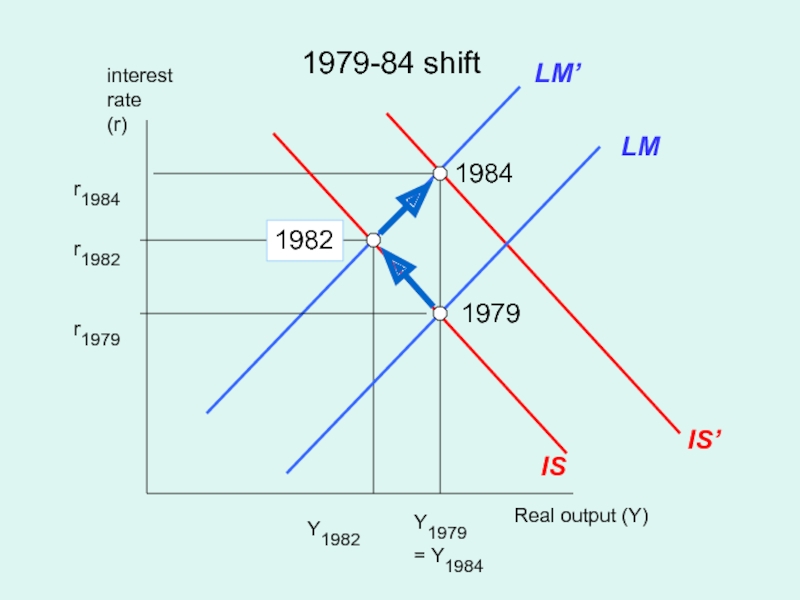
Слайд 30Case 2. What are the effects of fiscal policy?
A fiscal policy
shift is change in purchases (G) or in taxes (T), holding LM curve constant. See Figure.

interestrate(r)ISLMY*r*Fiscal expansionY*’r*’IS’")
interestrate(r)ISLMWhat is the multiplier?IS’μAB")
Слайд 33Multiplier Estimates by the CBO
Congressional Budget Office, Estimated Impact of the
ARRA, April 2010