- Главная
- Разное
- Дизайн
- Бизнес и предпринимательство
- Аналитика
- Образование
- Развлечения
- Красота и здоровье
- Финансы
- Государство
- Путешествия
- Спорт
- Недвижимость
- Армия
- Графика
- Культурология
- Еда и кулинария
- Лингвистика
- Английский язык
- Астрономия
- Алгебра
- Биология
- География
- Детские презентации
- Информатика
- История
- Литература
- Маркетинг
- Математика
- Медицина
- Менеджмент
- Музыка
- МХК
- Немецкий язык
- ОБЖ
- Обществознание
- Окружающий мир
- Педагогика
- Русский язык
- Технология
- Физика
- Философия
- Химия
- Шаблоны, картинки для презентаций
- Экология
- Экономика
- Юриспруденция
The Elasticity of supply and demand презентация
Содержание
- 1. The Elasticity of supply and demand
- 2. ELASTICITY: A MEASURE OF RESPONSE Imagine that
- 3. THE PRICE ELASTICITY OF DEMAND
- 4. NB: With a downward-sloping demand curve, price
- 5. COMPUTING THE PRICE ELASTICITY OF DEMAND
- 6. ARC ELASTISITY This measure of elasticity, which
- 7. IN OUR CASE The fact that
- 8. PRICE ELASTICITIES ALONG A LINEAR DEMAND
- 9. THE PRICE ELASTICITY OF DEMAND AND CHANGES
- 10. ELASTIC, UNIT ELASTIC, AND INELASTIC DEMAND To
- 11. For any linear demand curve, demand will
- 12. CONSTANT PRICE ELASTICITY OF DEMAND CURVES
- 13. DETERMINANTS OF THE PRICE ELASTICITY OF DEMAND
- 14. SUMMARY The price elasticity of demand measures
- 15. INCOME ELASTICITY OF DEMAND
- 17. CROSS PRICE ELASTICITY OF DEMAND
- 18. CROSS PRICE ELASTICITY OF DEMAND Cross price
- 19. SUMMARY The income elasticity of demand reflects
- 20. PRICE ELASTICITY OF SUPPLY Price elasticity
- 21. TYPES OF ELASTICITY Supply is price elastic
- 22. APPLICATION S2 – a supply curve in
- 23. SUMMARY The price elasticity of supply measures
Слайд 2ELASTICITY: A MEASURE OF RESPONSE
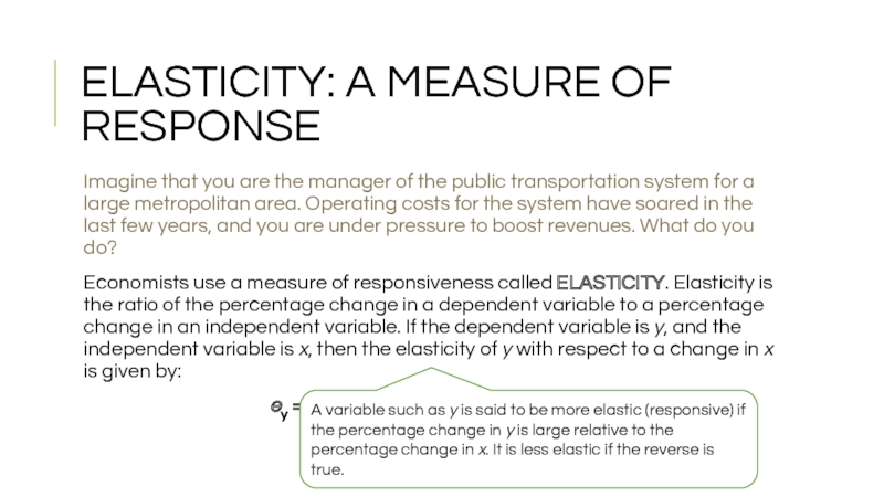
Imagine that you are the manager of
Economists use a measure of responsiveness called ELASTICITY. Elasticity is the ratio of the percentage change in a dependent variable to a percentage change in an independent variable. If the dependent variable is y, and the independent variable is x, then the elasticity of y with respect to a change in x is given by:
ey = (% change in y) /(% change in x)
A variable such as y is said to be more elastic (responsive) if the percentage change in y is large relative to the percentage change in x. It is less elastic if the reverse is true.
Слайд 4NB:
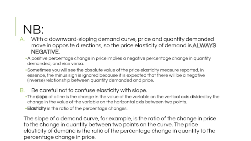
With a downward-sloping demand curve, price and quantity demanded move in
A positive percentage change in price implies a negative percentage change in quantity demanded, and vice versa.
Sometimes you will see the absolute value of the price elasticity measure reported. In essence, the minus sign is ignored because it is expected that there will be a negative (inverse) relationship between quantity demanded and price.
Be careful not to confuse elasticity with slope.
The slope of a line is the change in the value of the variable on the vertical axis divided by the change in the value of the variable on the horizontal axis between two points.
Elasticity is the ratio of the percentage changes.
The slope of a demand curve, for example, is the ratio of the change in price to the change in quantity between two points on the curve. The price elasticity of demand is the ratio of the percentage change in quantity to the percentage change in price.
Слайд 5COMPUTING THE PRICE ELASTICITY OF DEMAND
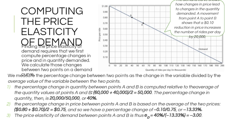
Finding the price elasticity of
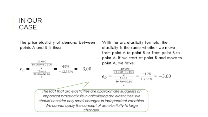
The demand curve shows how changes in price lead to changes in the quantity demanded. A movement from point A to point B shows that a $0.10 reduction in price increases the number of rides per day by 20,000.
We measure the percentage change between two points as the change in the variable divided by the average value of the variable between the two points.
the percentage change in quantity between points A and B is computed relative to theaverage of the quantity values at points A and B: (60,000 + 40,000)/2 = 50,000. The percentage change in quantity, then, is 20,000/50,000, or 40%.
the percentage change in price between points A and B is based on the average of the two prices: ($0.80 + $0.70)/2 = $0.75, and so we have a percentage change of −0.10/0.75, or −13.33%.
The price elasticity of demand between points A and B is thus eD = 40%/(−13.33%) = −3.00.
Слайд 6ARC ELASTISITY
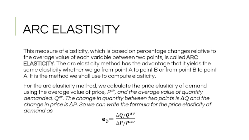
This measure of elasticity, which is based on percentage changes
For the arc elasticity method, we calculate the price elasticity of demand using the average value of price, Pav, and the average value of quantity demanded, Qav. The change in quantity between two points is ΔQ and the change in price is ΔP. So we can write the formula for the price elasticity of demand as
Слайд 7IN OUR CASE
The fact that arc elasticities are approximate suggests an
Слайд 8PRICE ELASTICITIES ALONG A LINEAR
DEMAND CURVE
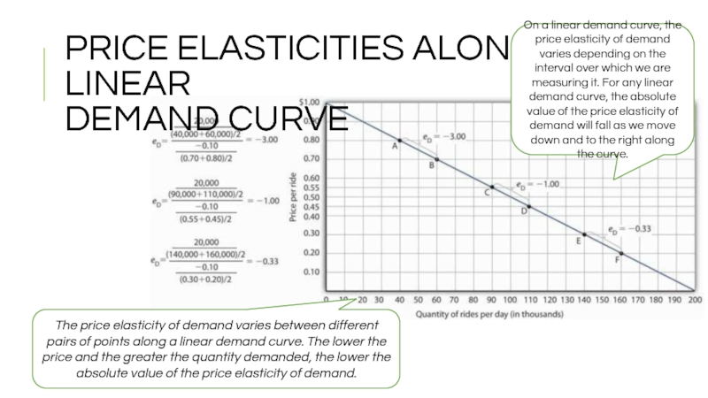
The price elasticity of demand
On a linear demand curve, the price elasticity of demand varies depending on the interval over which we are measuring it. For any linear demand curve, the absolute value of the price elasticity of demand will fall as we move down and to the right along the curve.
Слайд 9THE PRICE ELASTICITY OF DEMAND AND CHANGES IN TOTAL REVENUE
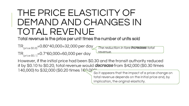
Total revenue
TR(price $0.8)=0.80*40,000=32,000 per day
TR(price $0.1)=0.7*60,000=60,000 per day
However, if the initial price had been $0.30 and the transit authority reduced it by $0.10 to $0.20, total revenue would decrease from $42,000 ($0.30 times 140,000) to $32,000 ($0.20 times 160,000).
The reduction in fare increases total revenue.
So it appears that the impact of a price change on total revenue depends on the initial price and, by implication, the original elasticity.
Слайд 10ELASTIC, UNIT ELASTIC, AND INELASTIC DEMAND
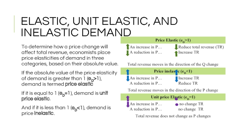
To determine how a price change
If the absolute value of the price elasticity of demand is greater than 1 (eD>1), demand is termed price elastic
If it is equal to 1 (eD=1), demand is unit price elastic.
And if it is less than 1 (eD<1), demand is price inelastic.
Слайд 11For any linear demand curve, demand will be price elastic in
Слайд 12CONSTANT PRICE ELASTICITY
OF DEMAND CURVES
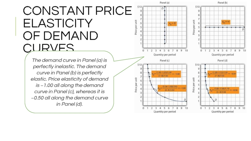
The demand curve in Panel (a)
Слайд 13DETERMINANTS OF THE PRICE ELASTICITY OF DEMAND
Availability of Substitutes (The availability
Importance in Household Budgets (One reason price changes affect quantity demanded is that they change how much a consumer can buy; a change in the price of a good or service affects the purchasing power of a consumer’s income and thus affects the amount of a good the consumer will buy. This effect is stronger when a good or service is important in a typical household’s budget.)
Time (depends in large part on how much time we allow for a response. the absolute value of the price elasticity of demand will be greater when more time is allowed for consumer responses.)
Слайд 14SUMMARY
The price elasticity of demand measures the responsiveness of quantity demanded
Demand is price inelastic if the absolute value of the price elasticity of demand is less than 1; it is unit price elastic if the absolute value is equal to 1; and it is price elastic if the absolute value is greater than 1.
Demand is price elastic in the upper half of any linear demand curve and price inelastic in the lower half. It is unit price elastic at the midpoint.
When demand is price inelastic, total revenue moves in the direction of a price change. When demand is unit price elastic, total revenue does not change in response to a price change. When demand is price elastic, total revenue moves in the direction of a quantity change.
The absolute value of the price elasticity of demand is greater when substitutes are available, when the good is important in household budgets, and when buyers have more time to adjust to changes in the price of the good.
Слайд 16
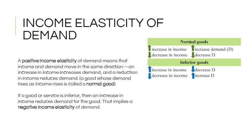
A positive income elasticity of demand means that income and demand
If a good or service is inferior, then an increase in income reduces demand for the good. That implies a negative income elasticity of demand.
INCOME ELASTICITY OF DEMAND
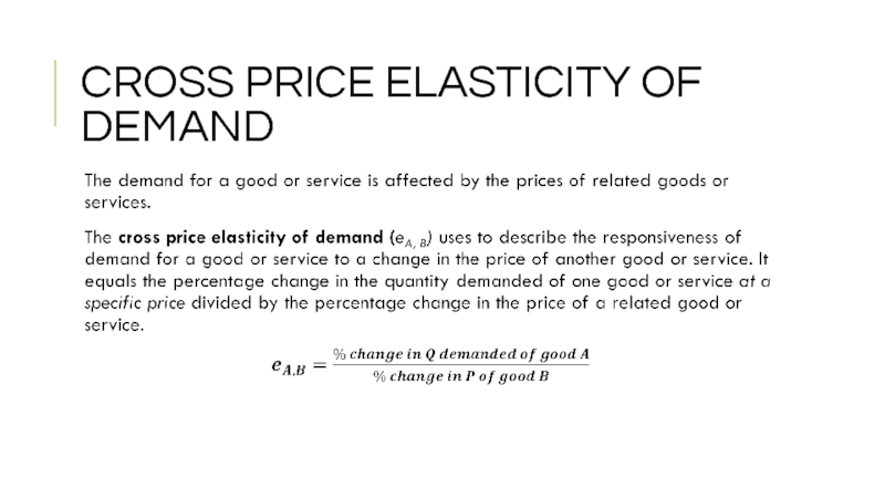
Слайд 18CROSS PRICE ELASTICITY OF DEMAND
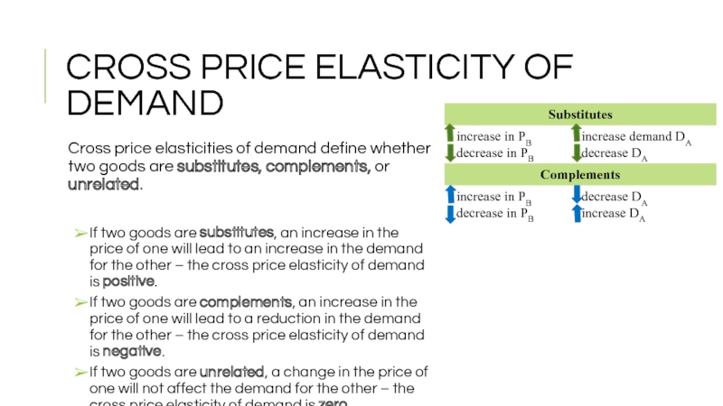
Cross price elasticities of demand define whether
If two goods are substitutes, an increase in the price of one will lead to an increase in the demand for the other – the cross price elasticity of demand is positive.
If two goods are complements, an increase in the price of one will lead to a reduction in the demand for the other – the cross price elasticity of demand is negative.
If two goods are unrelated, a change in the price of one will not affect the demand for the other – the cross price elasticity of demand is zero
Слайд 19SUMMARY
The income elasticity of demand reflects the responsiveness of demand to
Income elasticity is positive for normal goods and negative for inferior goods.
The cross price elasticity of demand measures the way demand for one good or service responds to changes in the price of another. It is the percentage change in the quantity demanded of one good or service at a specific price divided by the percentage change in the price of another good or service, all other things unchanged.
Cross price elasticity is positive for substitutes, negative for complements, and zero for goods or services whose demands are unrelated.
Слайд 20PRICE ELASTICITY OF SUPPLY
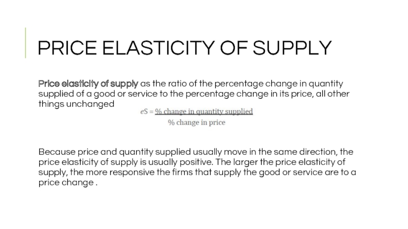
Price elasticity of supply as the ratio
Because price and quantity supplied usually move in the same direction, the price elasticity of supply is usually positive. The larger the price elasticity of supply, the more responsive the firms that supply the good or service are to a price change .
Слайд 21TYPES OF ELASTICITY
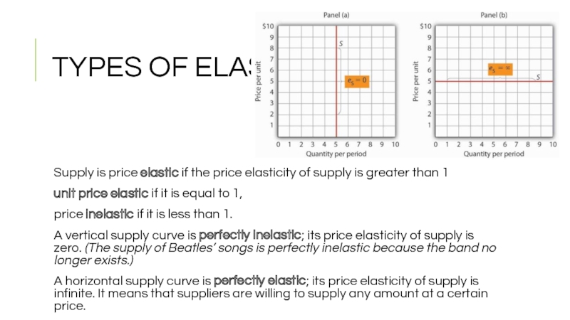
Supply is price elastic if the price elasticity of
unit price elastic if it is equal to 1,
price inelastic if it is less than 1.
A vertical supply curve is perfectly inelastic; its price elasticity of supply is zero. (The supply of Beatles’ songs is perfectly inelastic because the band no longer exists.)
A horizontal supply curve is perfectly elastic; its price elasticity of supply is infinite. It means that suppliers are willing to supply any amount at a certain price.
Слайд 22APPLICATION
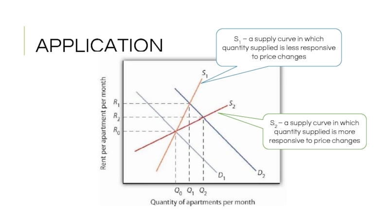
S2 – a supply curve in which quantity supplied is more
S1 – a supply curve in which quantity supplied is less responsive to price changes
Слайд 23SUMMARY
The price elasticity of supply measures the responsiveness of quantity supplied
Supply is price inelastic if the price elasticity of supply is less than 1; it is unit price elastic if the price elasticity of supply is equal to 1; and it is price elastic if the price elasticity of supply is greater than 1. A vertical supply curve is said to be perfectly inelastic. A horizontal supply curve is said to be perfectly elastic.
The price elasticity of supply is greater when the length of time under consideration is longer because over time producers have more options for adjusting to the change in price.
When applied to labor supply, the price elasticity of supply is usually positive but can be negative. If higher wages induce people to work more, the labor supply curve is upward sloping and the price elasticity of supply is positive. In some very high-paying professions, the labor supply curve may have a negative slope, which leads to a negative price elasticity of supply.
