- Главная
- Разное
- Дизайн
- Бизнес и предпринимательство
- Аналитика
- Образование
- Развлечения
- Красота и здоровье
- Финансы
- Государство
- Путешествия
- Спорт
- Недвижимость
- Армия
- Графика
- Культурология
- Еда и кулинария
- Лингвистика
- Английский язык
- Астрономия
- Алгебра
- Биология
- География
- Детские презентации
- Информатика
- История
- Литература
- Маркетинг
- Математика
- Медицина
- Менеджмент
- Музыка
- МХК
- Немецкий язык
- ОБЖ
- Обществознание
- Окружающий мир
- Педагогика
- Русский язык
- Технология
- Физика
- Философия
- Химия
- Шаблоны, картинки для презентаций
- Экология
- Экономика
- Юриспруденция
Monopoly Behavior презентация
Содержание
- 1. Monopoly Behavior
- 2. A Scotsman phones a dentist to inquire
- 3. — "I can't guarantee their professionalism and
- 4. How Should a Monopoly Price? So far
- 5. Capturing Consumer Surplus All pricing strategies we
- 6. Capturing Consumer Surplus Quantity $/Q The firm
- 7. Capturing Consumer Surplus Price discrimination is the
- 8. Price discrimination Price discrimination requires the absence of resale
- 9. Types of Price Discrimination 1st-degree: Each output
- 10. Types of Price Discrimination 3rd-degree: Price paid
- 11. First-degree Price Discrimination Each output unit is
- 12. First-degree Price Discrimination p(y) y $/output unit MC(y) Sell the th unit for $
- 13. First-degree Price Discrimination p(y) y $/output unit
- 14. First-degree Price Discrimination p(y) y $/output unit
- 15. First-degree Price Discrimination p(y) y $/output unit
- 16. First-degree Price Discrimination p(y) y $/output
- 17. First-degree Price Discrimination p(y) y $/output
- 18. Fig. 25.2
- 19. First-degree Price Discrimination First-degree price discrimination gives
- 20. First-Degree Price Discrimination In practice, perfect price
- 21. First-Degree Price Discrimination Examples of imperfect price
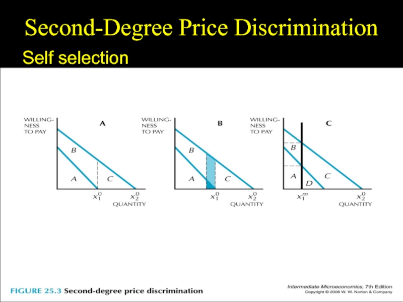
- 22. Second-Degree Price Discrimination In some markets, consumers
- 23. Second-Degree Price Discrimination Quantity discounts are an
- 24. Second-Degree Price Discrimination $/Q Without discrimination:
- 25. Fig. 25.3 Second-Degree Price Discrimination Self selection
- 26. Fig. 25.3 Second-Degree Price Discrimination Self selection
- 27. Fig. 25.3 Second-Degree Price Discrimination Self selection
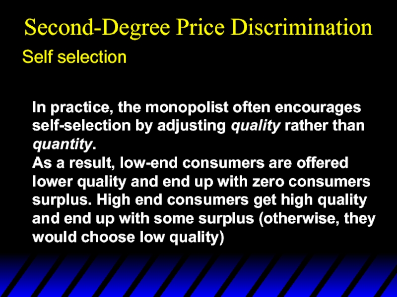
- 28. Fig. 25.3 Second-Degree Price Discrimination Self selection
- 29. Third-degree Price Discrimination Price paid by buyers
- 30. Third-degree Price Discrimination A monopolist manipulates market
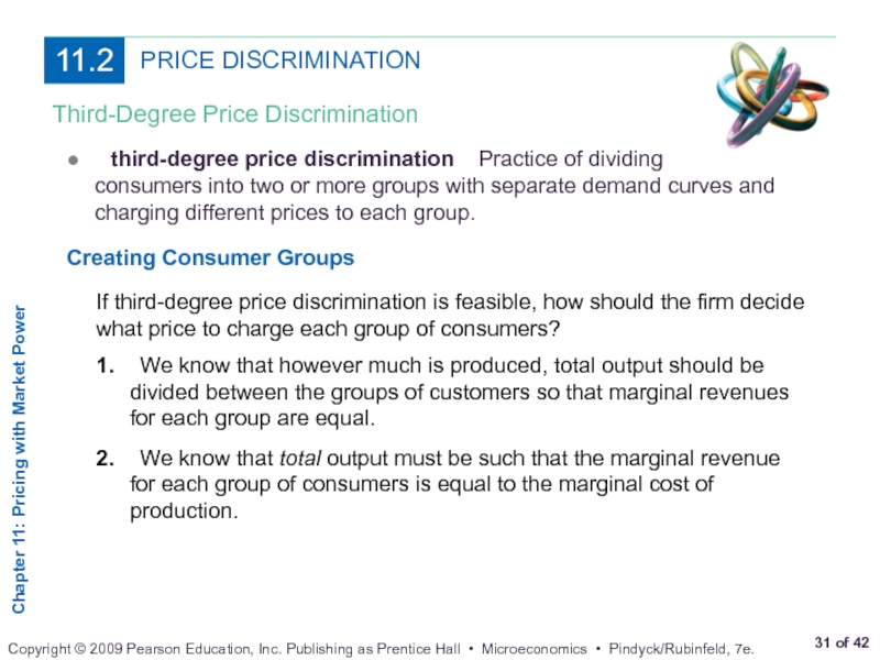
- 31. PRICE DISCRIMINATION Third-Degree Price Discrimination ● third-degree price
- 32. PRICE DISCRIMINATION Third-Degree Price Discrimination Creating Consumer Groups Determining Relative Prices
- 33. PRICE DISCRIMINATION Third-Degree Price Discrimination Third-Degree Price
- 34. Third-degree Price Discrimination
- 35. Third-degree Price Discrimination
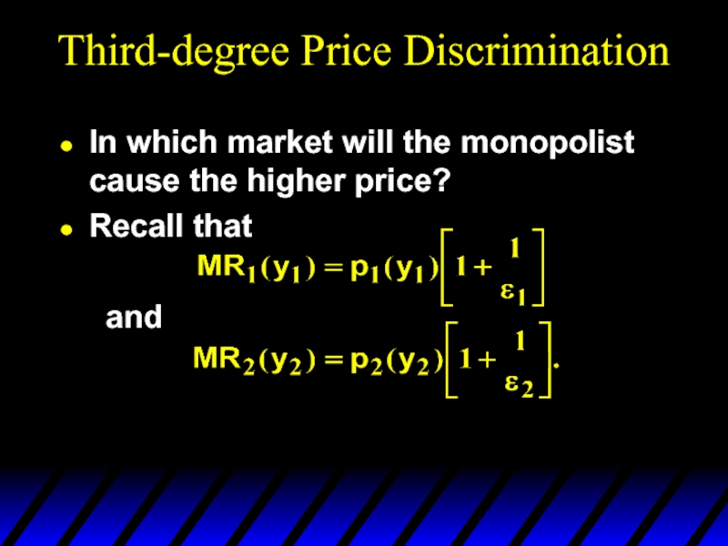
- 36. Third-degree Price Discrimination In which market will the monopolist cause the higher price?
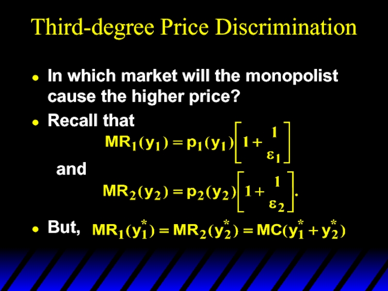
- 37. Third-degree Price Discrimination In which market will
- 38. Third-degree Price Discrimination In which market will
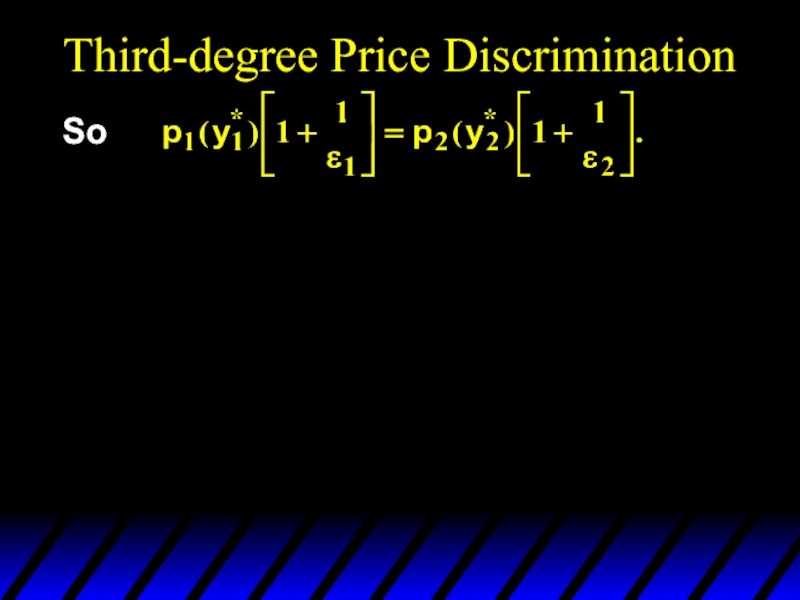
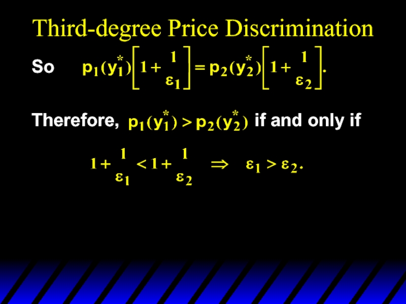
- 39. Third-degree Price Discrimination So
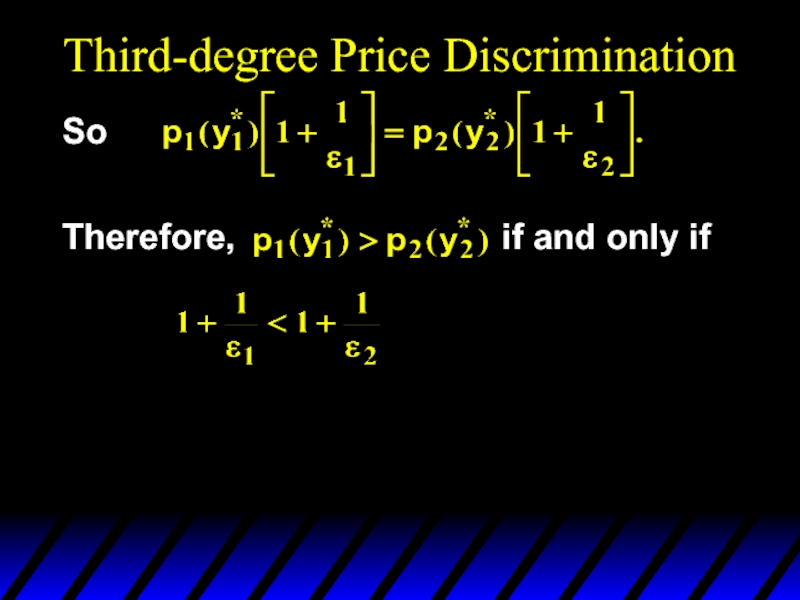
- 40. Third-degree Price Discrimination So Therefore,
- 41. Third-degree Price Discrimination So Therefore,
- 42. Third-degree Price Discrimination So Therefore,
- 43. No Sales to Smaller Market Even if
- 44. No Sales to Smaller Market Quantity $/Q
- 45. The Economics of Coupons
- 46. The Economics of Coupons and Rebates
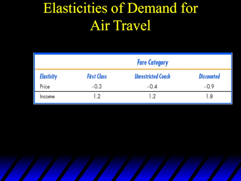
- 47. Price Elasticities of Demand: Users vs. Nonusers of Coupons
- 48. Airline Fares Differences in elasticities imply that
- 49. Elasticities of Demand for Air Travel
- 50. Airline Fares There are multiple fares for
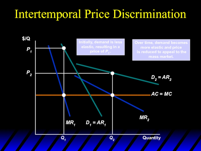
- 51. Other Types of Price Discrimination
- 52. Intertemporal Price Discrimination Once this market has
- 53. Intertemporal Price Discrimination Quantity $/Q Over time,
- 54. Other Types of Price Discrimination Peak-Load Pricing
- 55. Peak-Load Pricing Objective is to increase efficiency
- 56. Peak-Load Pricing With third-degree price discrimination, the
- 57. Peak-Load Pricing Quantity $/Q MR=MC for each
- 58. How to Price a Best-Selling Novel How
- 59. How to Price a Best-Selling Novel Company
- 60. How to Price a Best-Selling Novel Publishers
- 61. Two-Part Tariffs A two-part tariff is a
- 62. Two-Part Tariffs Should a monopolist prefer a
- 63. Two-Part Tariffs p1 + p2x Q: What is the largest that p1 can be?
- 64. Two-Part Tariffs p1 + p2x Q:
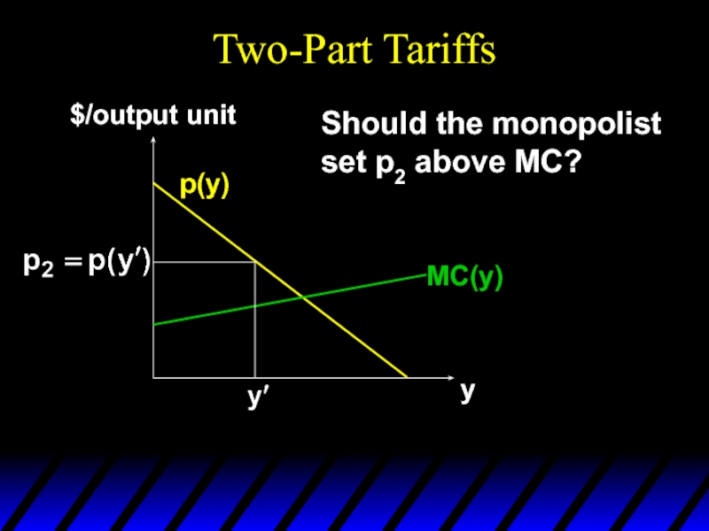
- 65. Two-Part Tariffs p(y) y $/output unit MC(y) Should the monopolist set p2 above MC?
- 66. Two-Part Tariffs p(y) y $/output unit
- 67. Two-Part Tariffs p(y) y $/output
- 68. Two-Part Tariffs p(y) y $/output unit
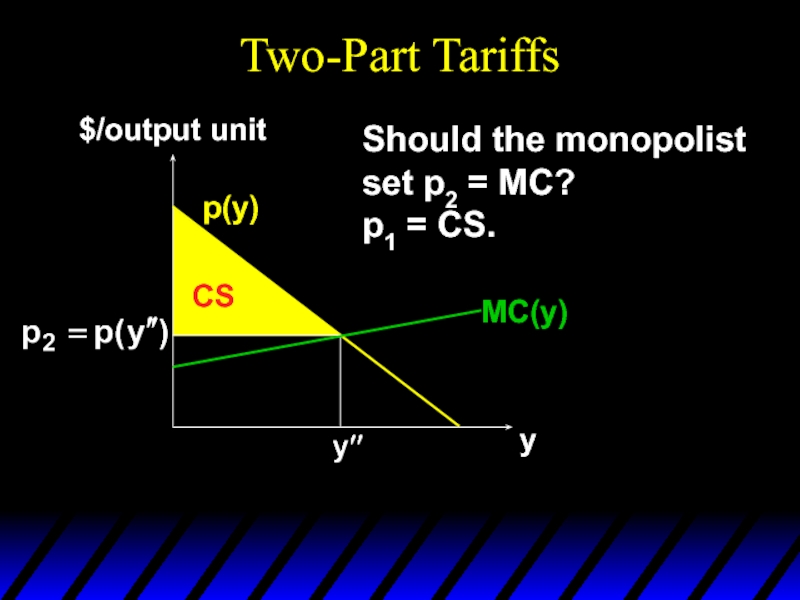
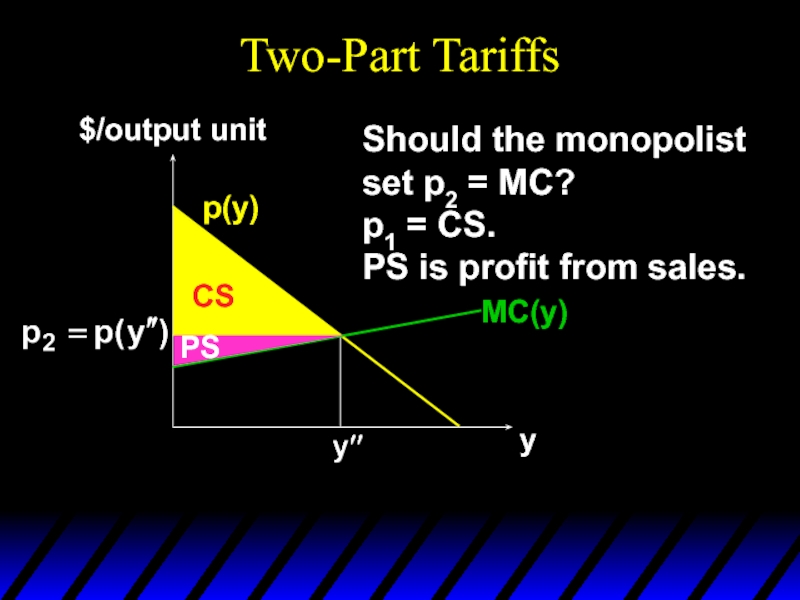
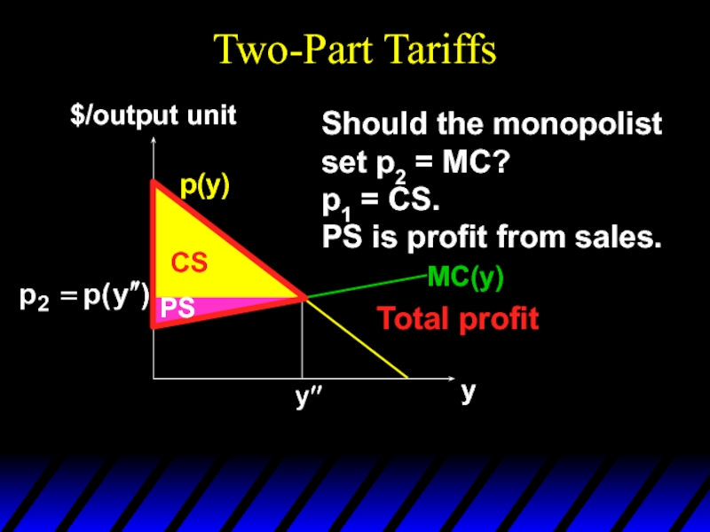
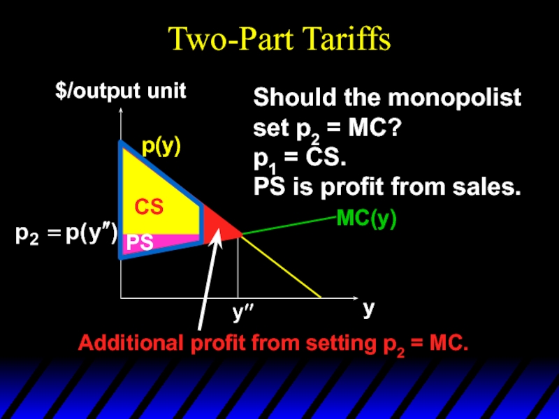
- 69. Two-Part Tariffs p(y) y $/output unit Should the monopolist set p2 = MC? MC(y)
- 70. Two-Part Tariffs p(y) y $/output unit
- 71. Two-Part Tariffs p(y) y $/output unit Should
- 72. Two-Part Tariffs p(y) y $/output
- 73. Two-Part Tariffs p(y) y $/output
- 74. Two-Part Tariffs p(y) y $/output
- 75. Two-Part Tariffs The monopolist maximizes its profit
- 76. Two-Part Tariffs A profit-maximizing two-part tariff gives
- 77. The Two-Part Tariff Form of pricing in
- 78. The Two-Part Tariff Pricing decision is setting
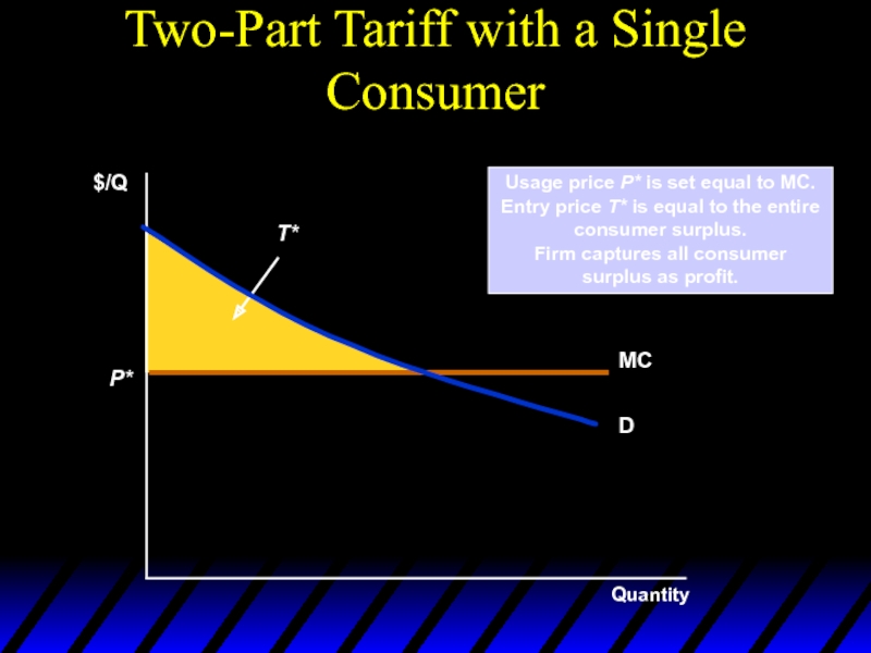
- 79. Usage price P* is set equal to
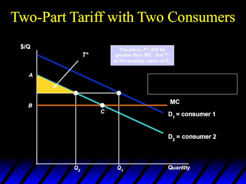
- 80. Two-Part Tariff with Two Consumers Two consumers,
- 81. The price, P*, will be greater
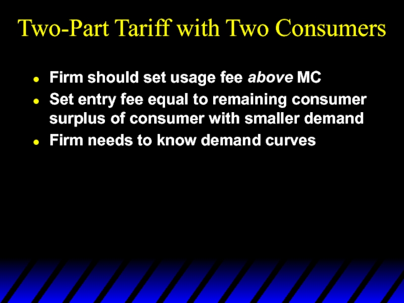
- 82. Two-Part Tariff with Two Consumers Firm should
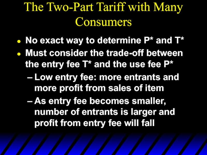
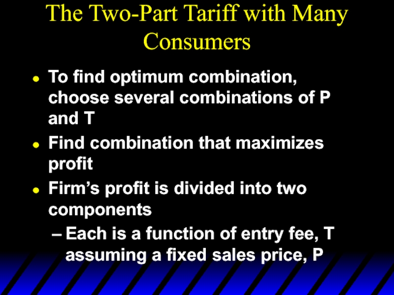
- 83. The Two-Part Tariff with Many Consumers No
- 84. The Two-Part Tariff with Many Consumers To
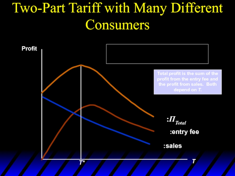
- 85. Two-Part Tariff with Many Different Consumers T
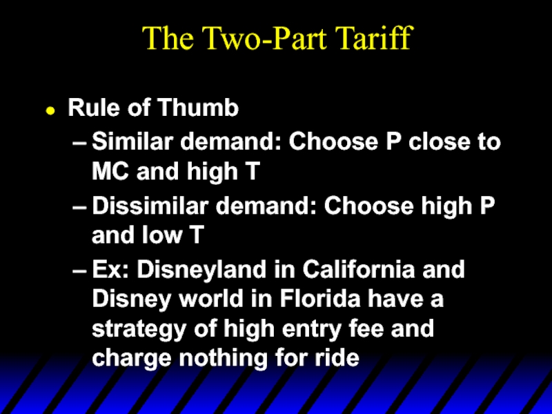
- 86. The Two-Part Tariff Rule of Thumb Similar
- 87. The Two-Part Tariff With a Twist Entry
- 88. Polaroid Cameras In 1971, Polaroid introduced the
- 89. Polaroid Cameras Buying camera is like entry
- 90. Polaroid Cameras Analytical framework:
- 91. Polaroid Cameras In the end, the film
- 92. Bundling Bundling is packaging two or more
- 93. Bundling When film company leased “Gone with
- 94. Bundling Renting the movies separately
- 95. Bundling If the movies are bundled: Theater
- 96. Relative Valuations More profitable to bundle because
- 97. Relative Valuations If the demands
- 98. Bundling If the movies are bundled: Theater
- 99. Bundling Bundling Scenario: Two different goods and
- 100. Reservation Prices r2 r1 For example,
- 101. Consumption Decisions When Products are Sold Separately
- 102. Consumption Decisions When Products are Bundled r2
- 103. Consumption Decisions When Products are Bundled The
- 104. Reservation Prices If the demands are
- 105. Reservation Prices r2 r1 If the demands
- 106. Movie Example r2 r1 Bundling pays due
- 107. Mixed Bundling Practice of selling two or
- 108. Mixed Versus Pure Bundling For each good,
- 109. Mixed Bundling – Example Demands are perfectly
- 110. Mixed Bundling – Example We can see
- 111. Bundling If MC is zero, mixed bundling
- 112. Mixed Bundling with Zero Marginal Costs A
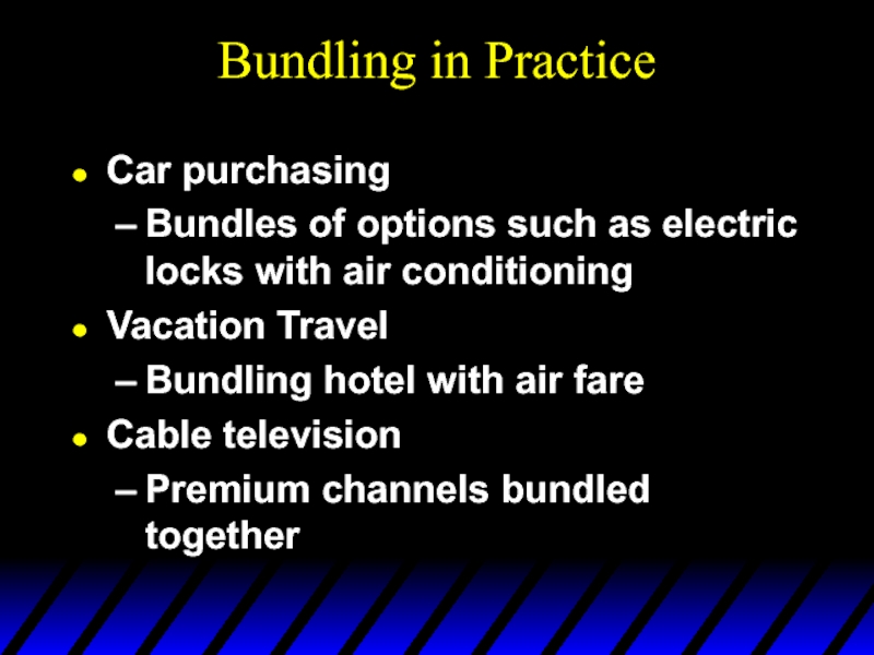
- 113. Bundling in Practice Car purchasing Bundles of
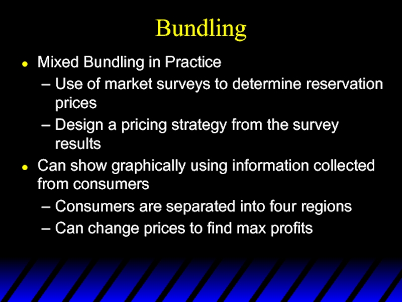
- 114. Bundling Mixed Bundling in Practice Use of
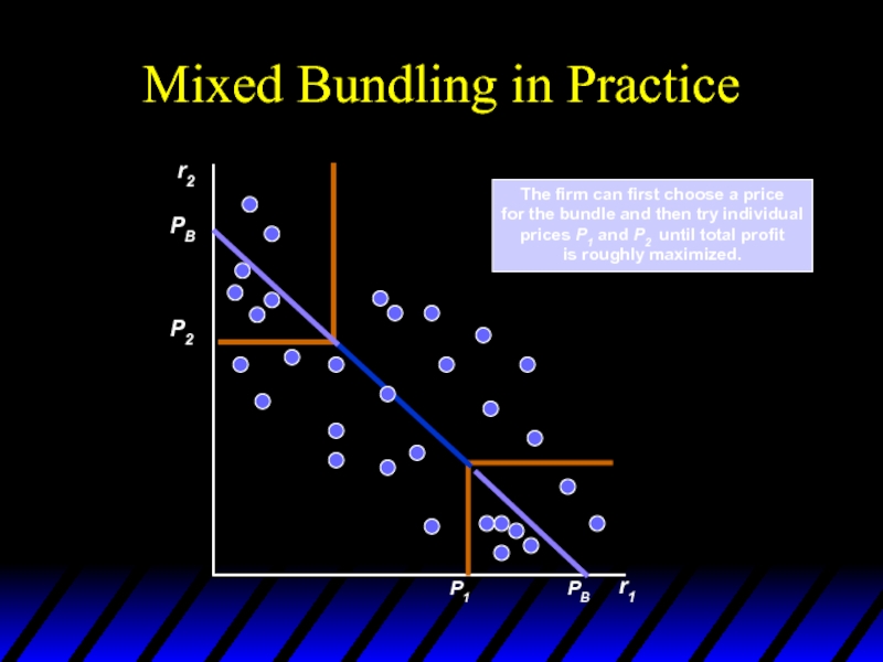
- 115. Mixed Bundling in Practice r2 r1 The
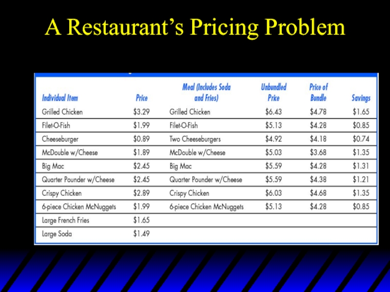
- 116. A Restaurant’s Pricing Problem
- 117. Tying The practice of requiring a customer
- 118. Tying Allows the seller to meter the
- 119. Versioning Extreme example: damaged goods Intel
- 120. Durable-goods pricing Waiting for the price cut.
- 121. Advertising Firms with market power have to
- 122. Advertising Assumptions Firm sets only one price
- 123. ADVERTISING Effects of Advertising Figure 11.20 AR
- 124. The price P and advertising expenditure A
- 125. First, rewrite equation (11.3) as follows: Now
- 126. Advertising A Rule of Thumb for Advertising
- 127. Advertising An Example R(Q) = $1 million/yr
- 128. Advertising The firm in our example should
- 129. Advertising – In Practice Estimate the level
Слайд 2A Scotsman phones a dentist to inquire about the cost for
— "85 pounds for an extraction, sir" the dentist replied.
** "85 quid ! Huv ye no'got anythin' cheaper ?„
— "That's the normal charge,” said the dentist.
** "Whit about if ye didn’t use any anesthetic ?„
— "That's unusual, sir, but I could do it and it would knock 15 pounds off".
** "What aboot if ye used one of your dentist trainees and still without any anesthetic ?"
Слайд 3— "I can't guarantee their professionalism and it'll be painful. But
** "How aboot if ye make it a trainin' session, have yer student do the extraction with the other students watchin' and learning‚?„
— "It'll be good for the students", mulled the dentist. "I'll charge you 5 pounds but it will be traumatic".
** " It's a deal,” said the Scotsman. "Can ye confirm an appointment for my wife next Tuesday then ?"
Слайд 4How Should a Monopoly Price?
So far a monopoly has been thought
Can price-discrimination earn a monopoly higher profits?
Слайд 5Capturing Consumer Surplus
All pricing strategies we will examine are means of
Profit maximizing point of P* and Q*
But some consumers will pay more than P* for a good
Raising price will lose some consumers, leading to smaller profits
Lowering price will gain some consumers, but lower profits
Слайд 6Capturing Consumer Surplus
Quantity
$/Q
The firm would like to charge higher price to
Firm would also like to sell to those in area B but without lowering price to all consumers
Both ways will allow the firm to capture more consumer surplus
Слайд 7Capturing Consumer Surplus
Price discrimination is the practice of charging different prices
Must be able to identify the different consumers and get them to pay different prices
Other techniques that expand the range of a firm’s market to get at more consumer surplus
Tariffs and bundling
Слайд 9Types of Price Discrimination
1st-degree: Each output unit is sold at a
2nd-degree: The price paid by a buyer can vary with the quantity demanded by the buyer. But all customers face the same price schedule. E.g., bulk-buying discounts.
Слайд 10Types of Price Discrimination
3rd-degree: Price paid by buyers in a given
Слайд 11First-degree Price Discrimination
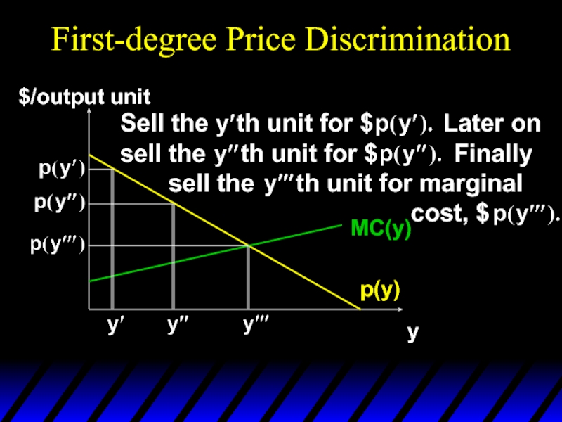
Each output unit is sold at a different price.
It requires that the monopolist can discover the buyer with the highest valuation of its product, the buyer with the next highest valuation, and so on.
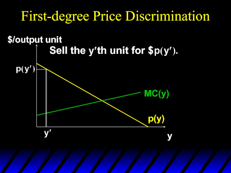
Слайд 13First-degree Price Discrimination
p(y)
y
$/output unit
MC(y)
Sell the th unit for $
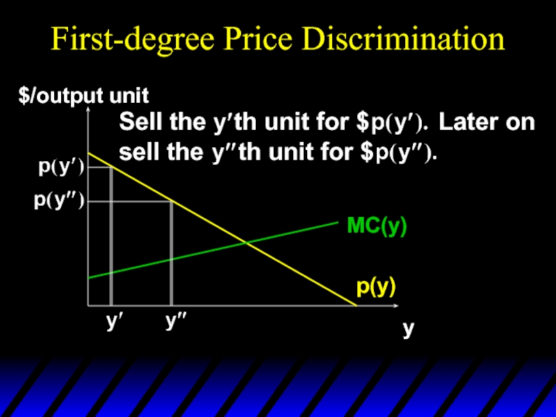
Слайд 14First-degree Price Discrimination
p(y)
y
$/output unit
MC(y)
Sell the th unit for $
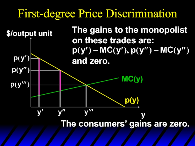
Слайд 15First-degree Price Discrimination
p(y)
y
$/output unit
MC(y)
The gains to the monopolist
on these trades are:
and
The consumers’ gains are zero.
Слайд 16
First-degree Price Discrimination
p(y)
y
$/output unit
MC(y)
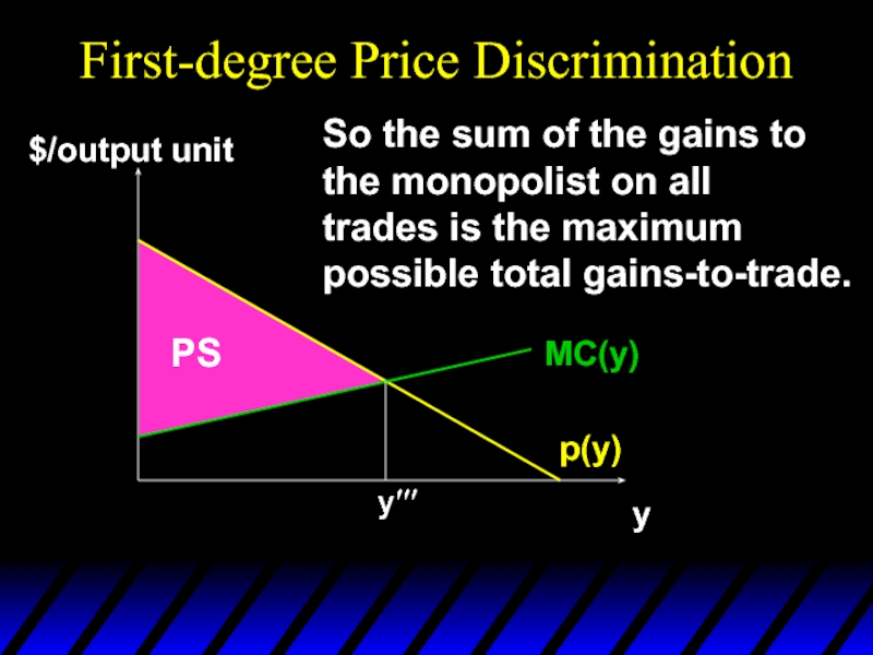
So the sum of the gains to
the monopolist
PS
Слайд 17
First-degree Price Discrimination
p(y)
y
$/output unit
MC(y)
The monopolist gets
the maximum possible
gains from
PS
First-degree price discrimination
is Pareto-efficient.
Слайд 19First-degree Price Discrimination
First-degree price discrimination gives a monopolist all of the
Слайд 20First-Degree Price Discrimination
In practice, perfect price discrimination is almost never possible
Impractical
Firms usually do not know reservation price of each customer
Firms can discriminate imperfectly
Can charge a few different prices based on some estimates of reservation prices
Слайд 21First-Degree Price Discrimination
Examples of imperfect price discrimination where the seller has
Lawyers, doctors, accountants, priests, policemen
Car salesperson (15% profit margin)
Colleges and universities (differences in financial aid)
Слайд 22Second-Degree Price Discrimination
In some markets, consumers purchase many units of a
Demand for that good declines with increased consumption
Electricity, water, heating fuel
Firms can engage in second-degree price discrimination
Practice of charging different prices per unit for different quantities of the same good or service
Слайд 23Second-Degree Price Discrimination
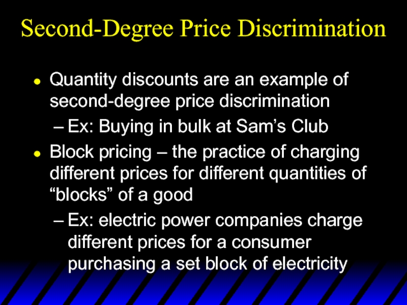
Quantity discounts are an example of second-degree price discrimination
Ex:
Block pricing – the practice of charging different prices for different quantities of “blocks” of a good
Ex: electric power companies charge different prices for a consumer purchasing a set block of electricity
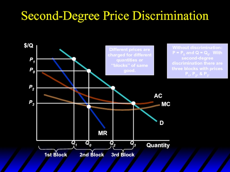
Слайд 24Second-Degree Price Discrimination
$/Q
Without discrimination:
P = P0 and Q = Q0.
Quantity
Different prices are charged for different quantities or “blocks” of same good.
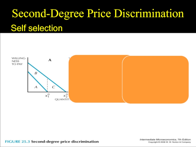
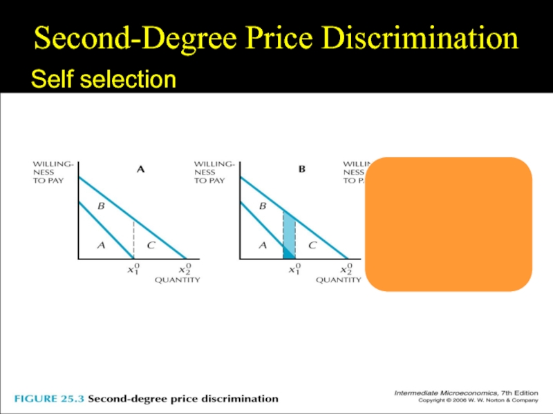
Слайд 28Fig. 25.3
Second-Degree Price Discrimination
Self selection
In practice, the monopolist often encourages self-selection
As a result, low-end consumers are offered lower quality and end up with zero consumers surplus. High end consumers get high quality and end up with some surplus (otherwise, they would choose low quality)
Слайд 29Third-degree Price Discrimination
Price paid by buyers in a given group is
Слайд 30Third-degree Price Discrimination
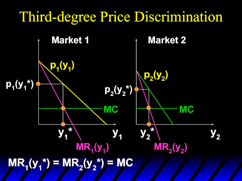
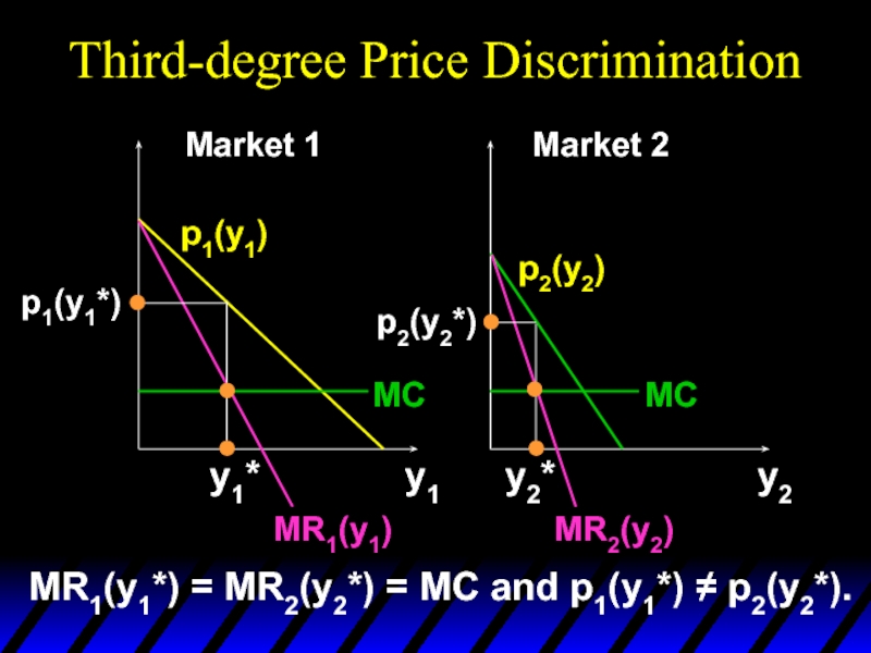
A monopolist manipulates market price by altering the quantity
So the question “What discriminatory prices will the monopolist set, one for each group?” is really the question “How many units of product will the monopolist supply to each group?”
Слайд 31PRICE DISCRIMINATION
Third-Degree Price Discrimination
● third-degree price discrimination Practice of dividing consumers
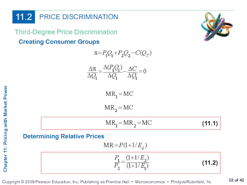
Creating Consumer Groups
If third-degree price discrimination is feasible, how should the firm decide what price to charge each group of consumers?
1. We know that however much is produced, total output should be divided between the groups of customers so that marginal revenues for each group are equal.
2. We know that total output must be such that the marginal revenue for each group of consumers is equal to the marginal cost of production.
Слайд 32PRICE DISCRIMINATION
Third-Degree Price Discrimination
Creating Consumer Groups
Determining Relative Prices
Слайд 33PRICE DISCRIMINATION
Third-Degree Price Discrimination
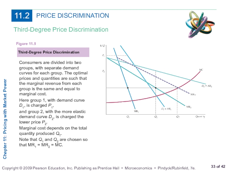
Third-Degree Price Discrimination
Figure 11.5
Consumers are divided into two
Here group 1, with demand curve D1, is charged P1,
and group 2, with the more elastic demand curve D2, is charged the lower price P2.
Marginal cost depends on the total quantity produced QT.
Note that Q1 and Q2 are chosen so that MR1 = MR2 = MC.
Слайд 34Third-degree Price Discrimination
MR1(y1)
MR2(y2)
y1
y2
y1*
y2*
p1(y1*)
p2(y2*)
MC
MC
p1(y1)
p2(y2)
Market 1
Market 2
MR1(y1*) = MR2(y2*) = MC
Слайд 35Third-degree Price Discrimination
MR1(y1)
MR2(y2)
y1
y2
y1*
y2*
p1(y1*)
p2(y2*)
MC
MC
p1(y1)
p2(y2)
Market 1
Market 2
MR1(y1*) = MR2(y2*) = MC and p1(y1*)
Слайд 36Third-degree Price Discrimination
In which market will the monopolist cause the higher
Слайд 37Third-degree Price Discrimination
In which market will the monopolist cause the higher
Recall that
and
Слайд 38Third-degree Price Discrimination
In which market will the monopolist cause the higher
Recall that
But,
and
Слайд 42Third-degree Price Discrimination
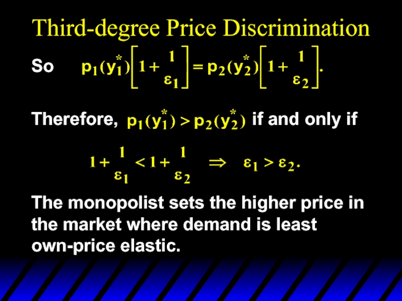
So
Therefore,
The monopolist sets the higher price in
the market where demand is least
own-price elastic.
Слайд 43No Sales to Smaller Market
Even if third-degree price discrimination is possible,
It is possible that the demand for one group is so low that it would not be profitable to lower price enough to sell to that group
Слайд 44No Sales to Smaller Market
Quantity
$/Q
Group one, with
demand D1, is not
for the good to make price discrimination profitable.
Слайд 45
The Economics of Coupons
and Rebates
Those consumers who are more price
Coupons and rebate programs allow firms to price discriminate
Слайд 46The Economics of Coupons
and Rebates
About 20 – 30% of consumers
Firms can get those with higher elasticities of demand to purchase the good who would not normally buy it
Table 11.1 shows how elasticities of demand vary for coupon/rebate users and non-users
Слайд 48Airline Fares
Differences in elasticities imply that some customers will pay a
Business travelers have few choices and their demand is less elastic
Casual travelers and families are more price-sensitive and will therefore be choosier
Слайд 50Airline Fares
There are multiple fares for every route flown by airlines
They
Must stay over a Saturday night
21-day advance, 14-day advance
Basic restrictions – can change ticket to only certain days
Most expensive: no restrictions – first class
Слайд 51
Other Types of Price Discrimination
Intertemporal Price Discrimination
Practice of separating consumers with
Initial release of a product, the demand is inelastic
Hard back vs. paperback book
New release movie
Technology
Слайд 52Intertemporal Price Discrimination
Once this market has yielded a maximum profit, firms
This can be seen graphically looking at two different groups of consumers – one willing to buy right now and one willing to wait
Слайд 53Intertemporal Price Discrimination
Quantity
$/Q
Over time, demand becomes
more elastic and price
is reduced
mass market.
Initially, demand is less
elastic, resulting in a
price of P1 .
Слайд 54Other Types of Price Discrimination
Peak-Load Pricing
Practice of charging higher prices during
Demand for some products may peak at particular times
Rush hour traffic
Electricity - late summer afternoons
Ski resorts on weekends
Слайд 55Peak-Load Pricing
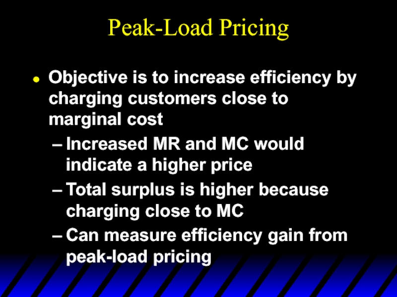
Objective is to increase efficiency by charging customers close to
Increased MR and MC would indicate a higher price
Total surplus is higher because charging close to MC
Can measure efficiency gain from peak-load pricing
Слайд 56Peak-Load Pricing
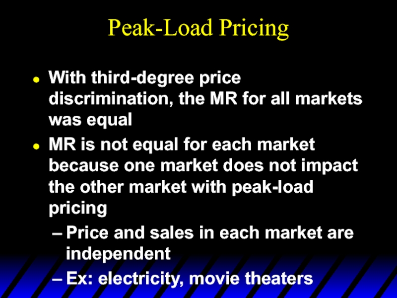
With third-degree price discrimination, the MR for all markets was
MR is not equal for each market because one market does not impact the other market with peak-load pricing
Price and sales in each market are independent
Ex: electricity, movie theaters
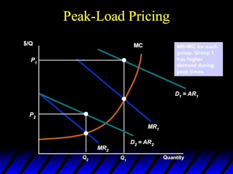
Слайд 57Peak-Load Pricing
Quantity
$/Q
MR=MC for each group. Group 1 has higher demand during
Слайд 58How to Price a Best-Selling Novel
How would you arrive at the
Hardback and paperback books are ways for the company to price discriminate
How does the company determine what price to sell the hardback and paperback books for?
How does the company determine when to release the paperback?
Слайд 59How to Price a Best-Selling Novel
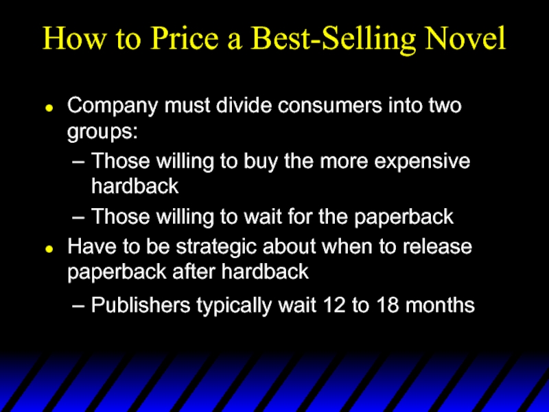
Company must divide consumers into two
Those willing to buy the more expensive hardback
Those willing to wait for the paperback
Have to be strategic about when to release paperback after hardback
Publishers typically wait 12 to 18 months
Слайд 60How to Price a Best-Selling Novel
Publishers must use estimates of past
Hard to determine the demand for a NEW book
New books are typically sold for about the same price, to take this into account
Demand for paperbacks is more elastic so we should expect it to be priced lower
Слайд 61Two-Part Tariffs
A two-part tariff is a lump-sum fee, p1, plus a
Thus the cost of buying x units of product is p1 + p2x.
Слайд 62Two-Part Tariffs
Should a monopolist prefer a two-part tariff to uniform pricing,
If so, how should the monopolist design its two-part tariff?
Слайд 64Two-Part Tariffs
p1 + p2x
Q: What is the largest that p1
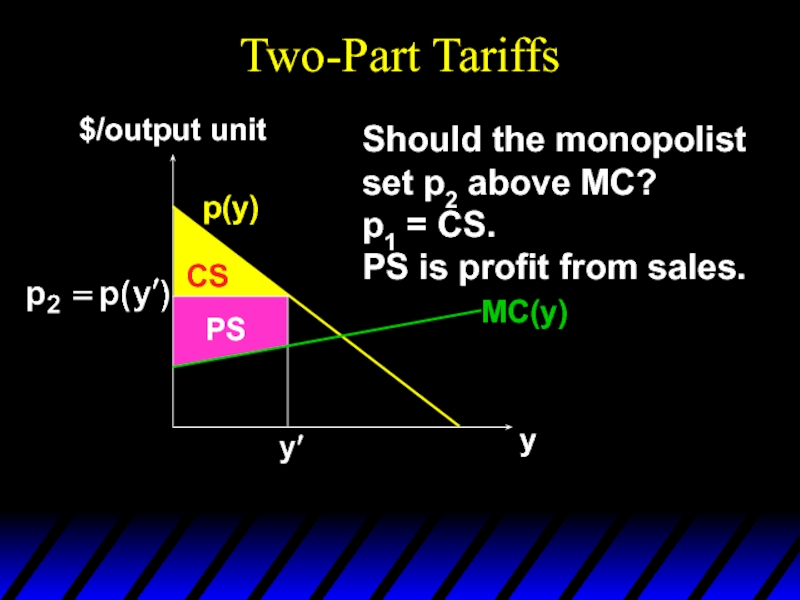
A: p1 is the “market entrance fee” so the largest it can be is the surplus the buyer gains from entering the market.
Set p1 = CS and now ask what should be p2?
Слайд 67
Two-Part Tariffs
p(y)
y
$/output unit
CS
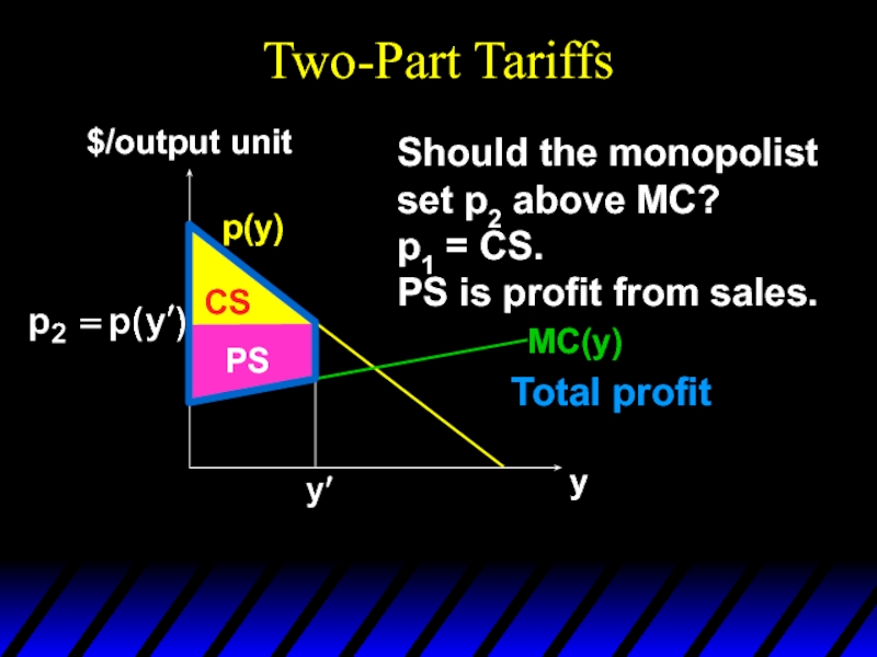
Should the monopolist
set p2 above MC?
p1 = CS.
PS is
MC(y)
PS
Слайд 68Two-Part Tariffs
p(y)
y
$/output unit
CS
Should the monopolist
set p2 above MC?
p1 = CS.
PS is
MC(y)
PS
Total profit
Слайд 71Two-Part Tariffs
p(y)
y
$/output unit
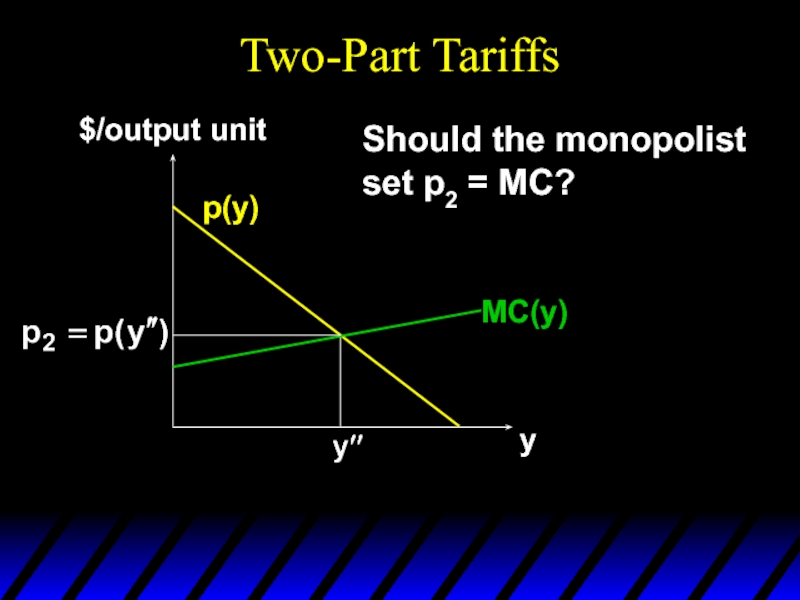
Should the monopolist
set p2 = MC?
p1 = CS.
PS is
MC(y)
CS
PS
Слайд 72
Two-Part Tariffs
p(y)
y
$/output unit
Should the monopolist
set p2 = MC?
p1 = CS.
PS is
MC(y)
CS
Total profit
PS
Слайд 73
Two-Part Tariffs
p(y)
y
$/output unit
Should the monopolist
set p2 = MC?
p1 = CS.
PS is
MC(y)
CS
PS
Слайд 74
Two-Part Tariffs
p(y)
y
$/output unit
Should the monopolist
set p2 = MC?
p1 = CS.
PS is
MC(y)
CS
Additional profit from setting p2 = MC.
PS
Слайд 75Two-Part Tariffs
The monopolist maximizes its profit when using a two-part tariff
Слайд 76Two-Part Tariffs
A profit-maximizing two-part tariff gives an efficient market outcome in
Слайд 77The Two-Part Tariff
Form of pricing in which consumers are charged both
Ex: amusement park, golf course, telephone service
A fee is charged upfront for right to use/buy the product
An additional fee is charged for each unit the consumer wishes to consume
Pay a fee to play golf and then pay another fee for each game you play
Слайд 78The Two-Part Tariff
Pricing decision is setting the entry fee (T) and
Choosing the trade-off between free-entry and high-use prices or high-entry and zero-use prices
Single Consumer
Assume firm knows consumer demand
Firm wants to capture as much consumer surplus as possible
Слайд 79Usage price P* is set equal to MC.
Entry price T*
Firm captures all consumer surplus as profit.
Two-Part Tariff with a Single Consumer
Quantity
$/Q
Слайд 80Two-Part Tariff with Two Consumers
Two consumers, but firm can only set
Does it make sense to set usage fee equal to MC and entrance fee equal to CS of the consumer with the smaller demand?
Слайд 81The price, P*, will be
greater than MC. Set T*
at
Two-Part Tariff with Two Consumers
Quantity
$/Q
Слайд 82Two-Part Tariff with Two Consumers
Firm should set usage fee above MC
Set
Firm needs to know demand curves
Слайд 83The Two-Part Tariff with Many Consumers
No exact way to determine P*
Must consider the trade-off between the entry fee T* and the use fee P*
Low entry fee: more entrants and more profit from sales of item
As entry fee becomes smaller, number of entrants is larger and profit from entry fee will fall
Слайд 84The Two-Part Tariff with Many Consumers
To find optimum combination, choose several
Find combination that maximizes profit
Firm’s profit is divided into two components
Each is a function of entry fee, T assuming a fixed sales price, P
Слайд 85Two-Part Tariff with Many Different Consumers
T
Profit
Total profit is the sum of
profit from the entry fee and
the profit from sales. Both
depend on T.
:ΠTotal
Слайд 86The Two-Part Tariff
Rule of Thumb
Similar demand: Choose P close to MC
Dissimilar demand: Choose high P and low T
Ex: Disneyland in California and Disney world in Florida have a strategy of high entry fee and charge nothing for ride
Слайд 87The Two-Part Tariff With a Twist
Entry price (T) entitles the buyer
Gillette razors sold with several blades
Amusement park admission comes with some tokens
On-line fees with free time
Can set higher entry fee without losing many consumers
Higher entry fee captures either surplus without driving them out of the market
Captures more surplus of large customers
Слайд 88Polaroid Cameras
In 1971, Polaroid introduced the SX-70 camera
Polaroid was able to
Allowed them greater profits than would have been possible if camera used ordinary film
Polaroid had a monopoly on cameras and film
Слайд 89Polaroid Cameras
Buying camera is like entry fee
Unlike an amusement park, for
It was necessary for Polaroid to have monopoly
If ordinary film could be used, the price of film would be close to MC
Polaroid needed to gain most of its profits from sale of film
Слайд 91Polaroid Cameras
In the end, the film prices were significantly above marginal
There was considerable heterogeneity of consumer demands
Слайд 92Bundling
Bundling is packaging two or more products to gain a pricing
Conditions necessary for bundling
Heterogeneous customers
Price discrimination is not possible
Demands must be negatively correlated
Слайд 93Bundling
When film company leased “Gone with the Wind,” it required theaters
Why would a company do this?
Company must be able to increase revenue
We can see the reservation prices for each theater and movie
Слайд 94
Bundling
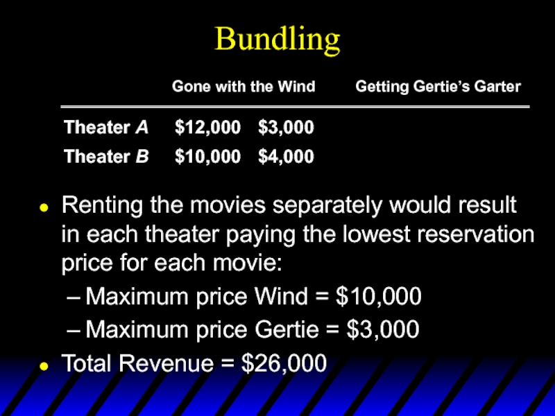
Renting the movies separately would result in each theater paying the
Maximum price Wind = $10,000
Maximum price Gertie = $3,000
Total Revenue = $26,000
Слайд 95Bundling
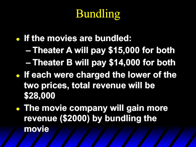
If the movies are bundled:
Theater A will pay $15,000 for both
Theater
If each were charged the lower of the two prices, total revenue will be $28,000
The movie company will gain more revenue ($2000) by bundling the movie
Слайд 96Relative Valuations
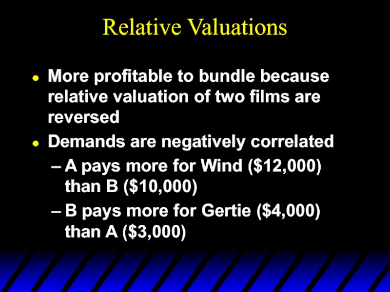
More profitable to bundle because relative valuation of two films
Demands are negatively correlated
A pays more for Wind ($12,000) than B ($10,000)
B pays more for Gertie ($4,000) than A ($3,000)
Слайд 97
Relative Valuations
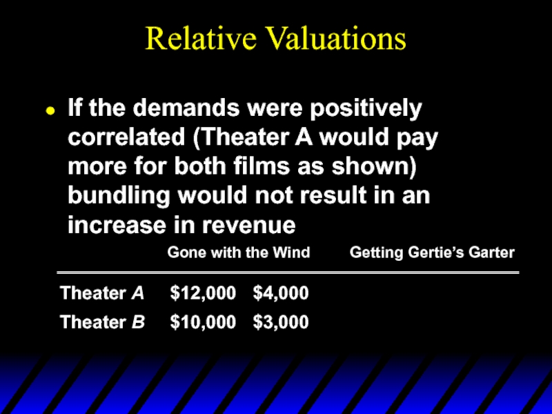
If the demands were positively correlated (Theater A would pay
Слайд 98Bundling
If the movies are bundled:
Theater A will pay $16,000 for both
Theater
If each were charged the lower of the two prices, total revenue will be $26,000, the same as by selling the films separately
Слайд 99Bundling
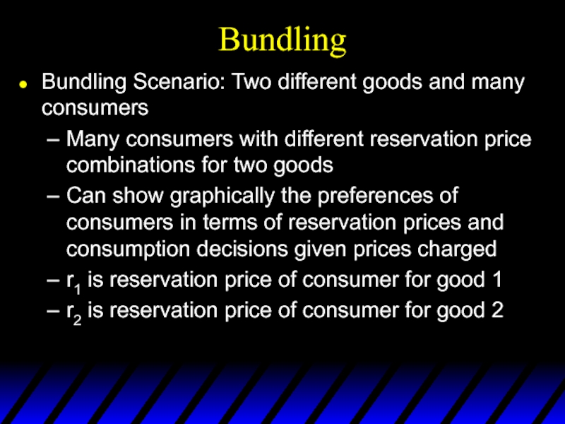
Bundling Scenario: Two different goods and many consumers
Many consumers with different
Can show graphically the preferences of consumers in terms of reservation prices and consumption decisions given prices charged
r1 is reservation price of consumer for good 1
r2 is reservation price of consumer for good 2
Слайд 100Reservation Prices
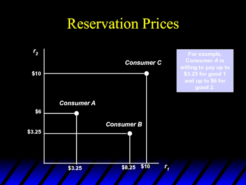
r2
r1
For example, Consumer A is willing to pay up
Слайд 101Consumption Decisions When
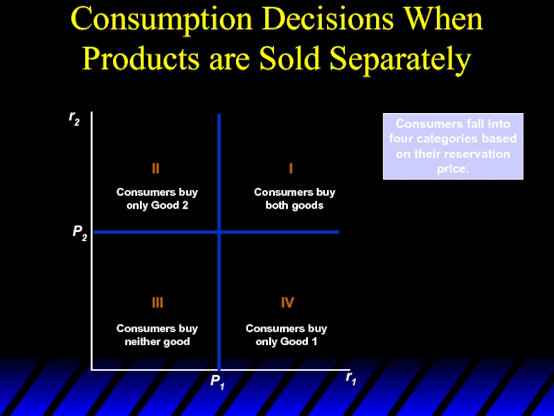
Products are Sold Separately
r2
r1
Consumers fall into
four categories based
on their
price.
Слайд 102Consumption Decisions When Products are Bundled
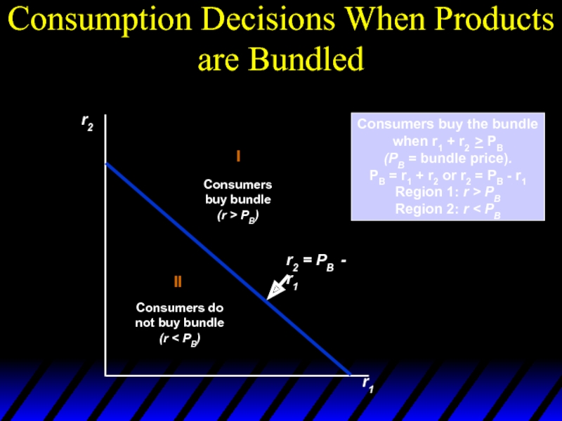
r2
r1
Consumers buy the bundle
when r1 +
(PB = bundle price).
PB = r1 + r2 or r2 = PB - r1
Region 1: r > PB
Region 2: r < PB
Слайд 103Consumption Decisions
When Products are Bundled
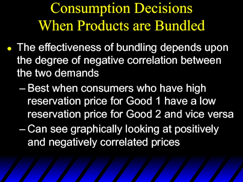
The effectiveness of bundling depends upon the
Best when consumers who have high reservation price for Good 1 have a low reservation price for Good 2 and vice versa
Can see graphically looking at positively and negatively correlated prices
Слайд 104Reservation Prices
If the demands are
perfectly positively
correlated, the firm
will not gain
It would earn the same
profit by selling the
goods separately.
Слайд 105Reservation Prices
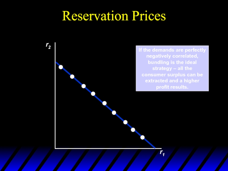
r2
r1
If the demands are perfectly negatively correlated, bundling is the
consumer surplus can be extracted and a higher
profit results.
Слайд 106Movie Example
r2
r1
Bundling pays due to
negative correlation.
(Wind)
(Gertie)
5,000
14,000
10,000
5,000
10,000
14,000
Слайд 107Mixed Bundling
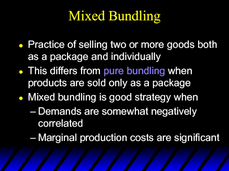
Practice of selling two or more goods both as a
This differs from pure bundling when products are sold only as a package
Mixed bundling is good strategy when
Demands are somewhat negatively correlated
Marginal production costs are significant
Слайд 108Mixed Versus Pure Bundling
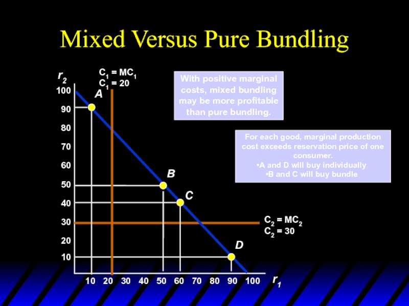
For each good, marginal production cost exceeds reservation
A and D will buy individually
B and C will buy bundle
With positive marginal
costs, mixed bundling
may be more profitable
than pure bundling.
Слайд 109Mixed Bundling – Example
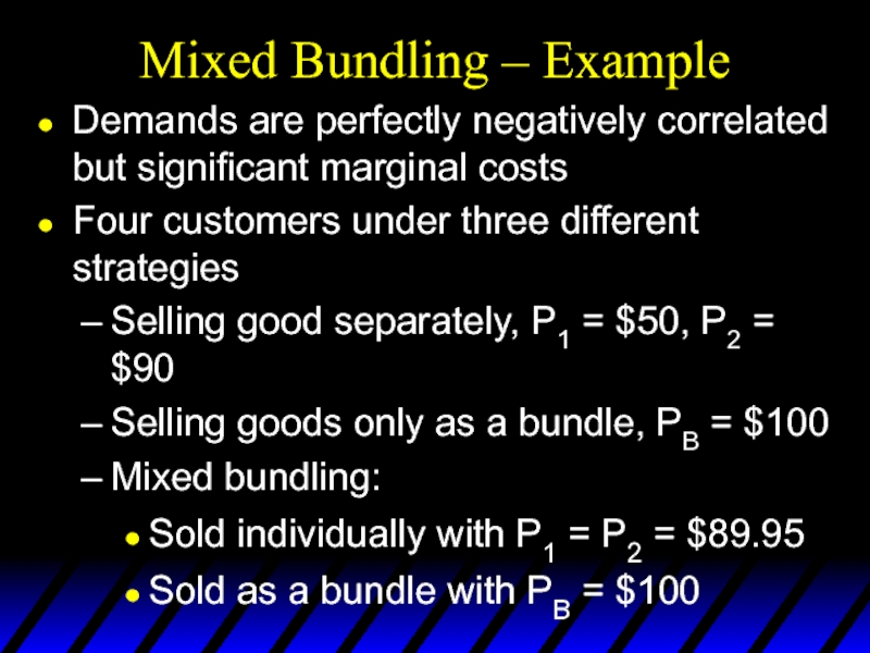
Demands are perfectly negatively correlated but significant marginal
Four customers under three different strategies
Selling good separately, P1 = $50, P2 = $90
Selling goods only as a bundle, PB = $100
Mixed bundling:
Sold individually with P1 = P2 = $89.95
Sold as a bundle with PB = $100
Слайд 110Mixed Bundling – Example
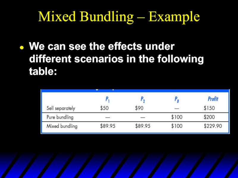
We can see the effects under different scenarios
Слайд 111Bundling
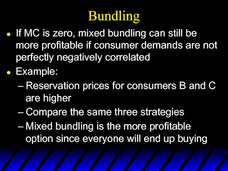
If MC is zero, mixed bundling can still be more profitable
Example:
Reservation prices for consumers B and C are higher
Compare the same three strategies
Mixed bundling is the more profitable option since everyone will end up buying
Слайд 112Mixed Bundling with Zero Marginal Costs
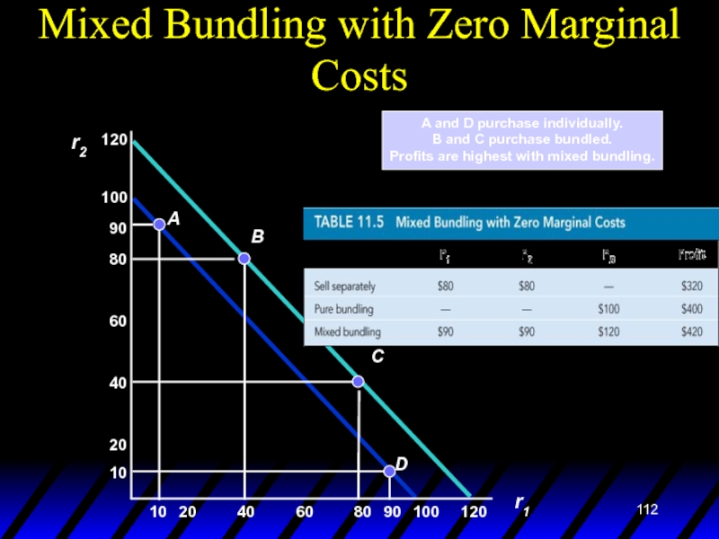
A and D purchase individually.
B and
Profits are highest with mixed bundling.
Слайд 113Bundling in Practice
Car purchasing
Bundles of options such as electric locks with
Vacation Travel
Bundling hotel with air fare
Cable television
Premium channels bundled together
Слайд 114Bundling
Mixed Bundling in Practice
Use of market surveys to determine reservation prices
Design
Can show graphically using information collected from consumers
Consumers are separated into four regions
Can change prices to find max profits
Слайд 115Mixed Bundling in Practice
r2
r1
The firm can first choose a price
for the
prices P1 and P2 until total profit
is roughly maximized.
P2
PB
PB
P1
Слайд 117Tying
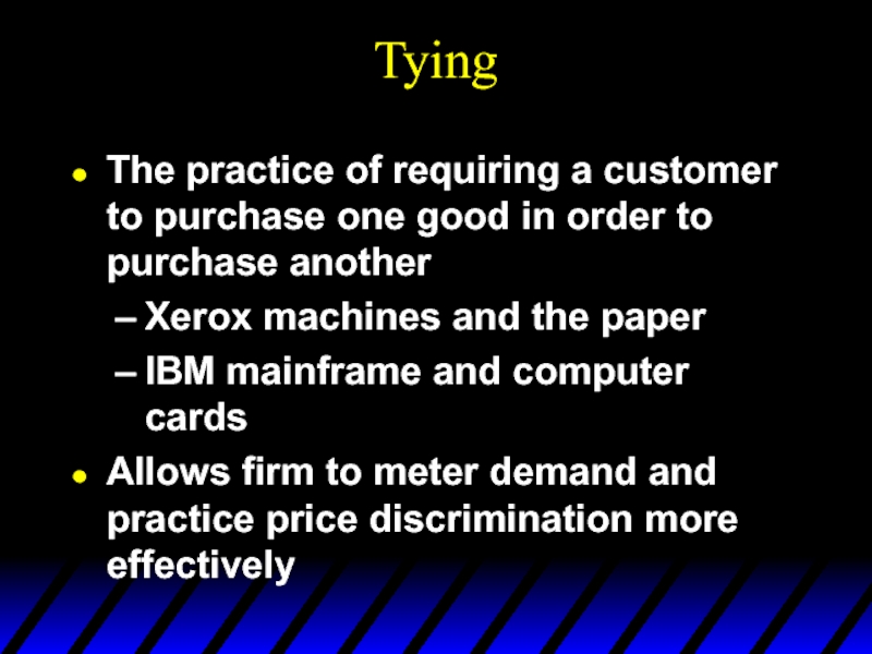
The practice of requiring a customer to purchase one good in
Xerox machines and the paper
IBM mainframe and computer cards
Allows firm to meter demand and practice price discrimination more effectively
Слайд 118Tying
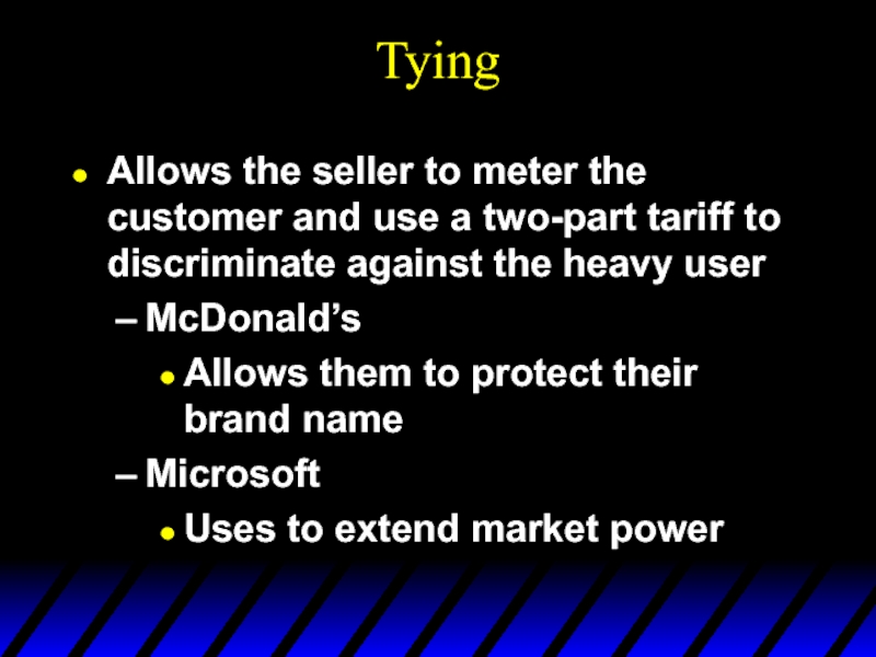
Allows the seller to meter the customer and use a two-part
McDonald’s
Allows them to protect their brand name
Microsoft
Uses to extend market power
Слайд 119Versioning
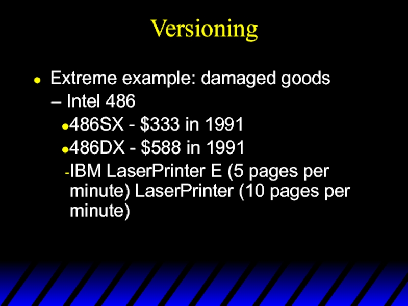
Extreme example: damaged goods
Intel 486
486SX - $333 in 1991
486DX -
IBM LaserPrinter E (5 pages per minute) LaserPrinter (10 pages per minute)
Слайд 120Durable-goods pricing
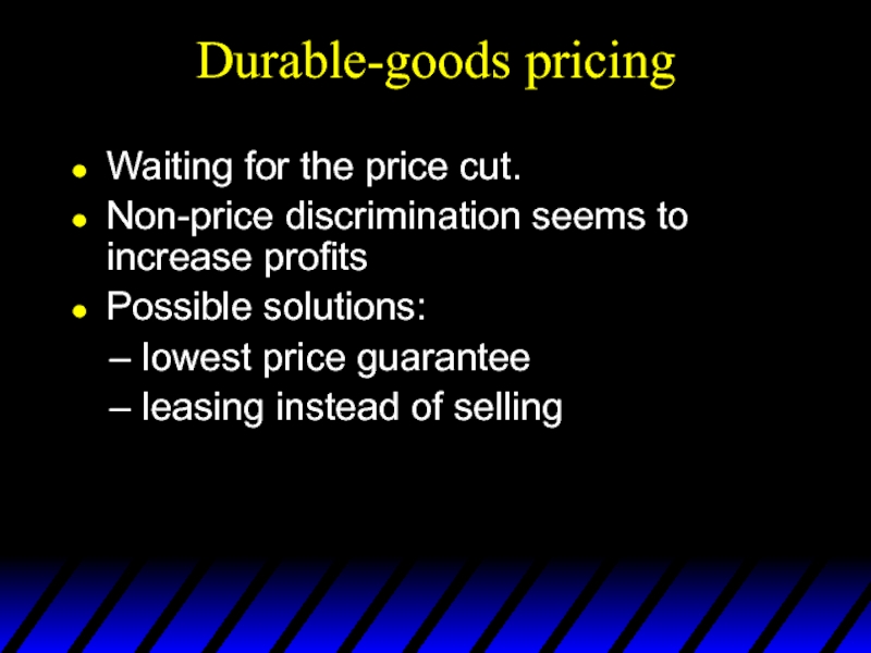
Waiting for the price cut.
Non-price discrimination seems to increase profits
Possible
lowest price guarantee
leasing instead of selling
Слайд 121Advertising
Firms with market power have to decide how much to advertise
We
Decision depends on characteristics of demand for firm’s product
Слайд 122Advertising
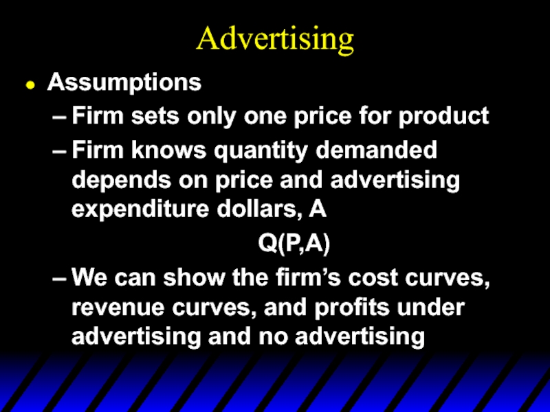
Assumptions
Firm sets only one price for product
Firm knows quantity demanded depends
Q(P,A)
We can show the firm’s cost curves, revenue curves, and profits under advertising and no advertising
Слайд 123ADVERTISING
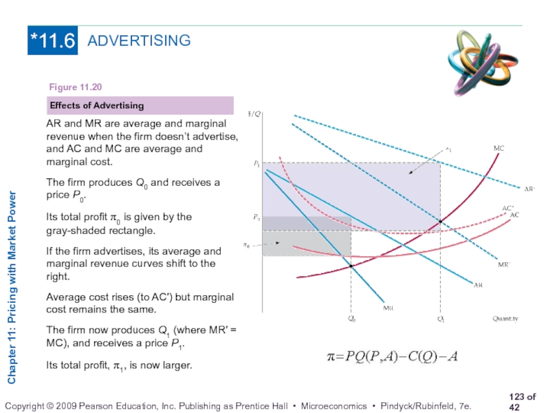
Effects of Advertising
Figure 11.20
AR and MR are average and marginal revenue
and AC and MC are average and marginal cost.
The firm produces Q0 and receives a price P0.
Its total profit π0 is given by the gray-shaded rectangle.
If the firm advertises, its average and marginal revenue curves shift to the right.
Average cost rises (to AC′) but marginal cost remains the same.
The firm now produces Q1 (where MR′ = MC), and receives a price P1.
Its total profit, π1, is now larger.
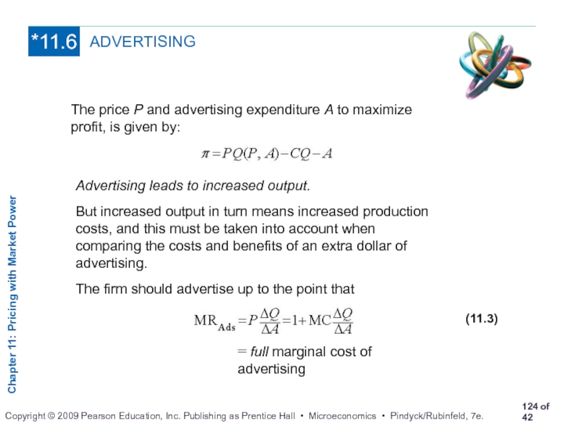
Слайд 124The price P and advertising expenditure A to maximize profit, is
The firm should advertise up to the point that
= full marginal cost of advertising
(11.3)
Advertising leads to increased output.
But increased output in turn means increased production costs, and this must be taken into account when comparing the costs and benefits of an extra dollar of advertising.
ADVERTISING
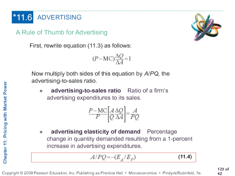
Слайд 125First, rewrite equation (11.3) as follows:
Now multiply both sides of this
● advertising-to-sales ratio Ratio of a firm’s advertising expenditures to its sales.
● advertising elasticity of demand Percentage change in quantity demanded resulting from a 1-percent increase in advertising expenditures.
A Rule of Thumb for Advertising
ADVERTISING
Слайд 126Advertising
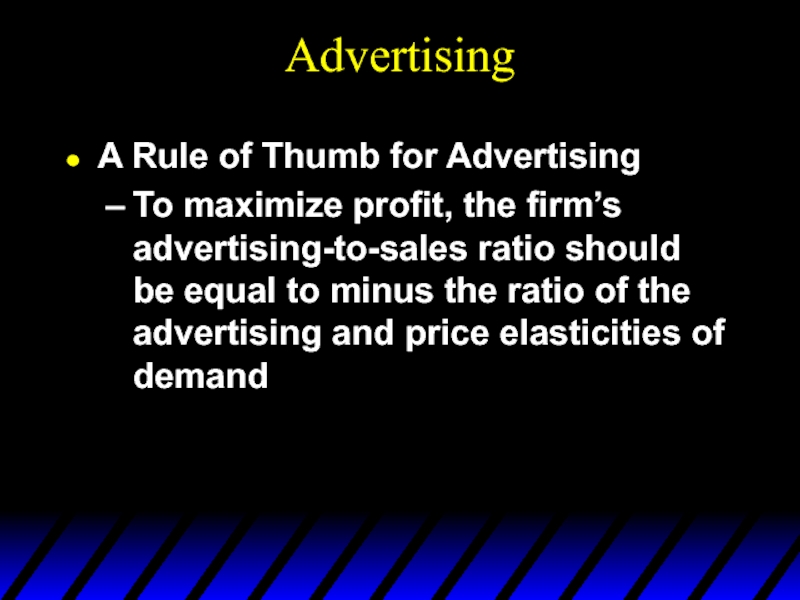
A Rule of Thumb for Advertising
To maximize profit, the firm’s advertising-to-sales
Слайд 127Advertising
An Example
R(Q) = $1 million/yr
$10,000 budget for A (advertising--1% of revenues)
EA
EP = -4 (markup price over MC is substantial)
Слайд 128Advertising
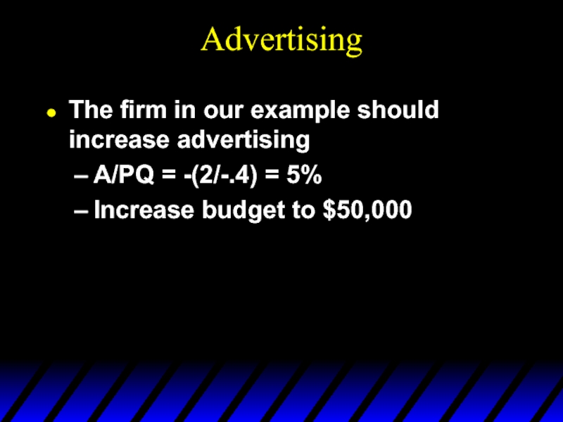
The firm in our example should increase advertising
A/PQ = -(2/-.4) =
Increase budget to $50,000
Слайд 129Advertising – In Practice
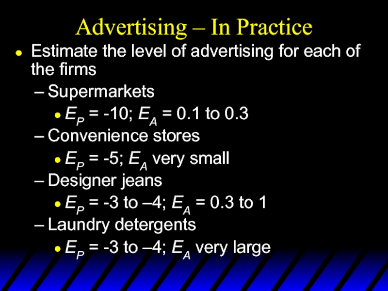
Estimate the level of advertising for each of
Supermarkets
EP = -10; EA = 0.1 to 0.3
Convenience stores
EP = -5; EA very small
Designer jeans
EP = -3 to –4; EA = 0.3 to 1
Laundry detergents
EP = -3 to –4; EA very large
