- Главная
- Разное
- Дизайн
- Бизнес и предпринимательство
- Аналитика
- Образование
- Развлечения
- Красота и здоровье
- Финансы
- Государство
- Путешествия
- Спорт
- Недвижимость
- Армия
- Графика
- Культурология
- Еда и кулинария
- Лингвистика
- Английский язык
- Астрономия
- Алгебра
- Биология
- География
- Детские презентации
- Информатика
- История
- Литература
- Маркетинг
- Математика
- Медицина
- Менеджмент
- Музыка
- МХК
- Немецкий язык
- ОБЖ
- Обществознание
- Окружающий мир
- Педагогика
- Русский язык
- Технология
- Физика
- Философия
- Химия
- Шаблоны, картинки для презентаций
- Экология
- Экономика
- Юриспруденция
Lecture # 09. Inputs and Production Functions презентация
Содержание
- 1. Lecture # 09. Inputs and Production Functions
- 2. Outline The Production Function Marginal and Average
- 3. Definitions Inputs or factors of production are
- 4. Definitions Production transforms a set of inputs
- 5. Definitions The production function tells us the
- 6. Definitions A technically efficient firm is attaining
- 7. Example: The Production Function and Technical Efficiency L Q • C
- 8. Example: The Production Function and Technical Efficiency L Q • • C D
- 9. Example: The Production Function and Technical Efficiency
- 10. Example: The Production Function and Technical Efficiency
- 11. Example: The Production Function and Technical
- 12. Notes: The variables in the production function
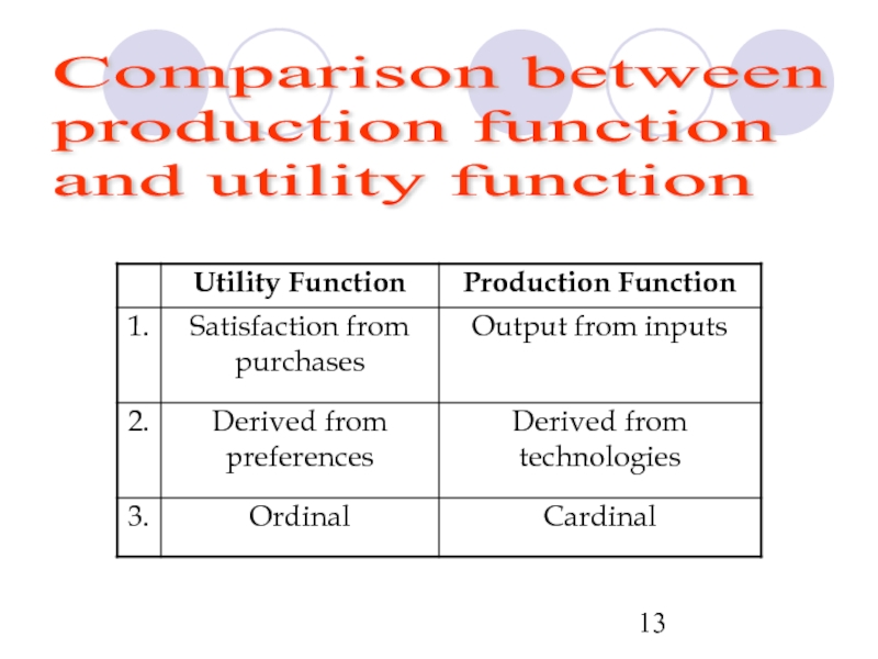
- 13. Comparison between production function and utility function
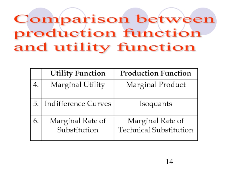
- 14. Comparison between production function and utility function
- 15. Marginal Product Definition: The marginal product of
- 16. Example: Suppose Q = K0.5L0.5 Then:
- 17. Average Product Definition: The average product of
- 18. Example: Suppose Q = K0.5L0.5 Then:
- 19. Law of Diminishing Marginal Returns Definition: The
- 20. Q L Q= F(L,K0) Example: Total and Marginal Product
- 21. Q L MPL maximized Q=
- 22. Q L MPL = 0
- 23. Example: Total and Marginal Product
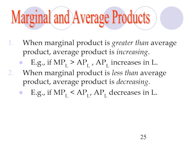
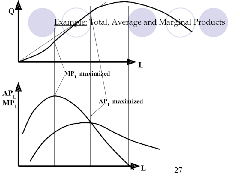
- 24. Marginal and Average Products There is a
- 25. Marginal and Average Products When marginal product
- 26. Example: Average and Marginal Products L APL MPL MPL maximized APL maximized
- 27. Example: Total, Average and Marginal Products
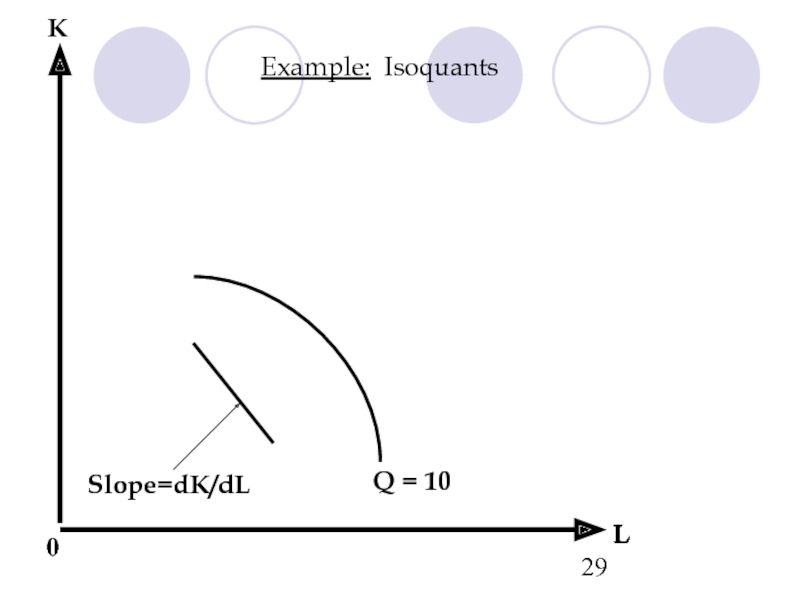
- 28. Isoquants Definition: An isoquant is a representation
- 29. Example: Isoquants L K Q = 10 0 Slope=dK/dL L
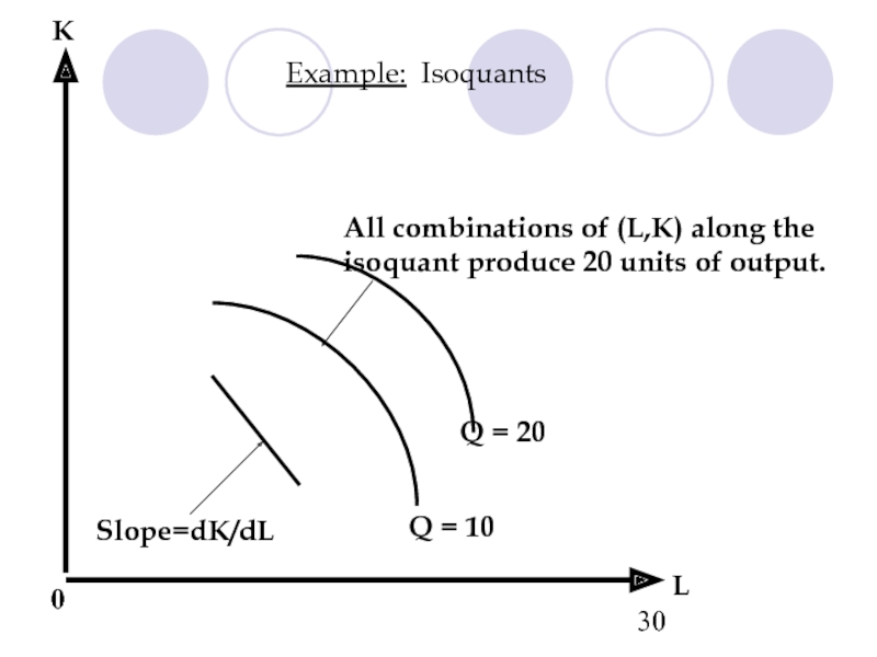
- 30. L Q = 10 Q = 20
- 31. Isoquants Example: Suppose Q = K0.5L0.5
- 32. Definition: The marginal rate of technical substitution
- 33. Marginal Rate Of Technical Substitution Alternative
- 34. Marginal Product and the Marginal Rate
- 35. Marginal Product and the Marginal Rate
- 36. Marginal Product and the Marginal Rate
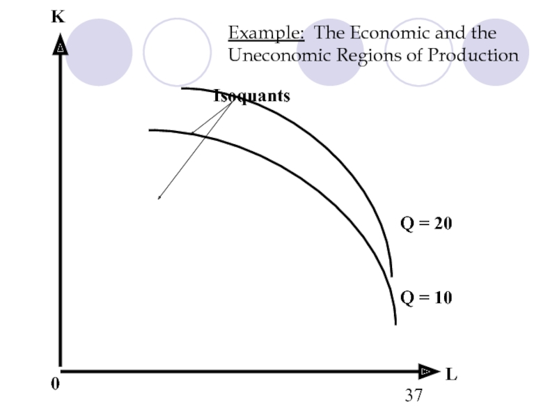
- 37. Example: The Economic and the Uneconomic Regions
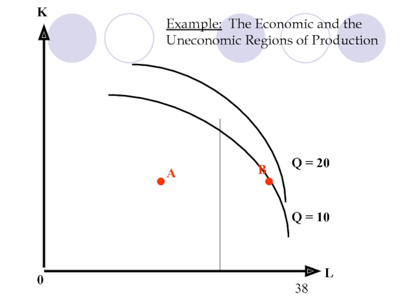
- 38. Example: The Economic and the Uneconomic Regions
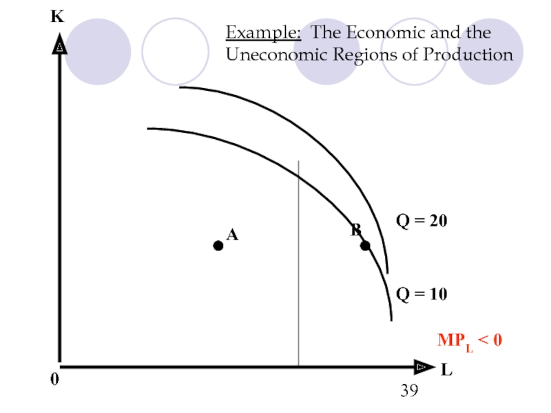
- 39. Example: The Economic and the Uneconomic Regions
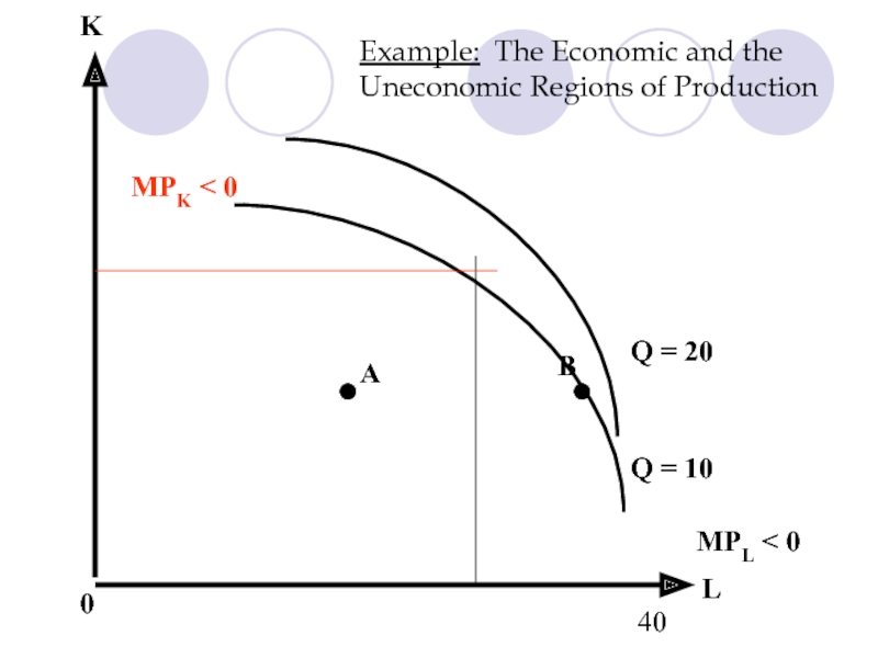
- 40. Example: The Economic and the Uneconomic Regions
- 41. Example: The Economic and the
- 42. Example: The Economic and
Слайд 2Outline
The Production Function
Marginal and Average Products
Isoquants
Marginal Rate of Technical Substitution
Returns to
Some Special Functional Forms
Technological Progress
Слайд 3Definitions
Inputs or factors of production are productive resources that firms use
Example: labor, land, capital equipment…
The firm’s output is the amount of goods and services produced by the firm.
Слайд 4Definitions
Production transforms a set of inputs into a set of outputs
Technology
Слайд 5Definitions
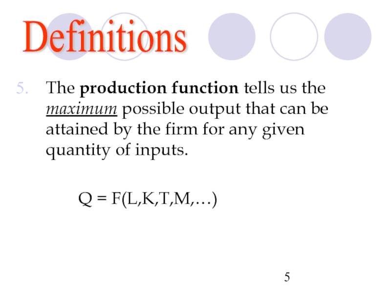
The production function tells us the maximum possible output that can
Q = F(L,K,T,M,…)
Слайд 6Definitions
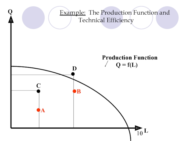
A technically efficient firm is attaining the maximum possible output from
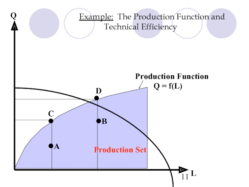
The firm’s production set is the set of all feasible points, including:
The production function (efficient point)
The inefficient points below the production function
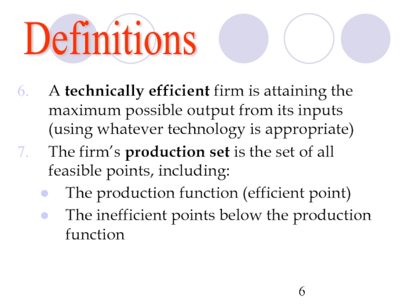
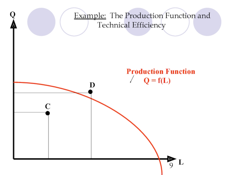
Слайд 10Example: The Production Function and Technical Efficiency
Q = f(L)
L
Q
•
•
•
•
C
D
A
B
Production Function
Слайд 11
Example: The Production Function and Technical Efficiency
Q = f(L)
L
Q
•
•
•
•
C
D
A
B
Production Set
Production
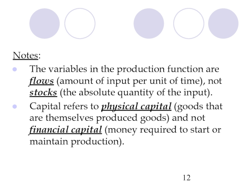
Слайд 12Notes:
The variables in the production function are flows (amount of input
Capital refers to physical capital (goods that are themselves produced goods) and not financial capital (money required to start or maintain production).
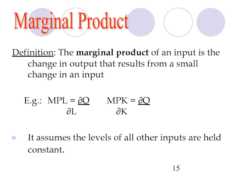
Слайд 15Marginal Product
Definition: The marginal product of an input is the change
E.g.: MPL = ∂Q MPK = ∂Q
∂L ∂K
It assumes the levels of all other inputs are held constant.
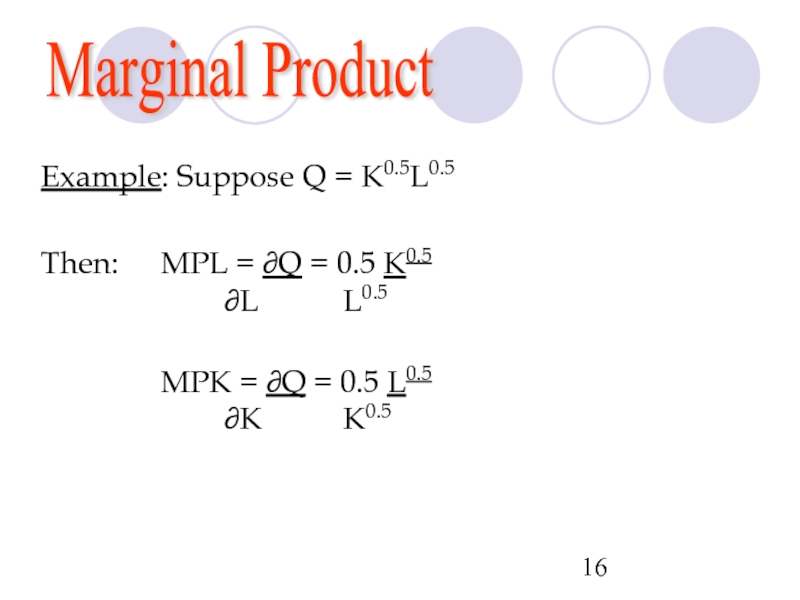
Слайд 16Example: Suppose Q = K0.5L0.5
Then: MPL = ∂Q = 0.5 K0.5
MPK = ∂Q = 0.5 L0.5
∂K K0.5
Marginal Product
Слайд 17Average Product
Definition: The average product of an input is equal to
E.g.: APL = Q APK = Q
L K
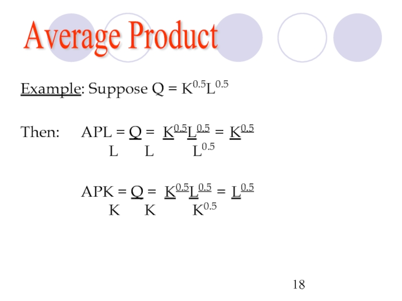
Слайд 18Example: Suppose Q = K0.5L0.5
Then: APL = Q = K0.5L0.5 =
L L L0.5
APK = Q = K0.5L0.5 = L0.5
K K K0.5
Average Product
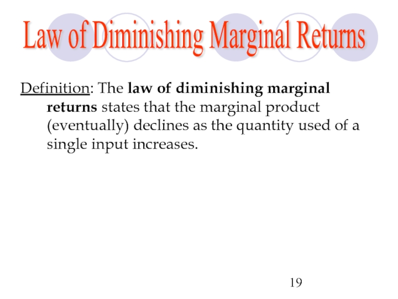
Слайд 19Law of Diminishing Marginal Returns
Definition: The law of diminishing marginal returns
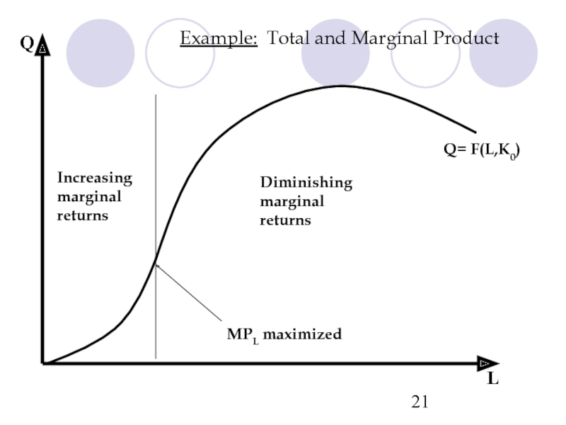
Слайд 21Q
L
MPL maximized
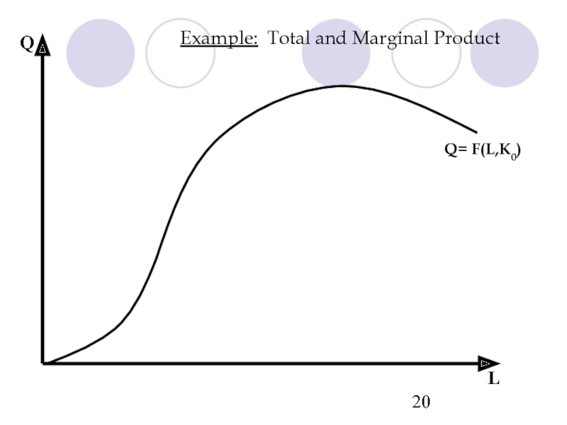
Q= F(L,K0)
Example: Total and Marginal Product
Increasing marginal returns
Diminishing marginal returns
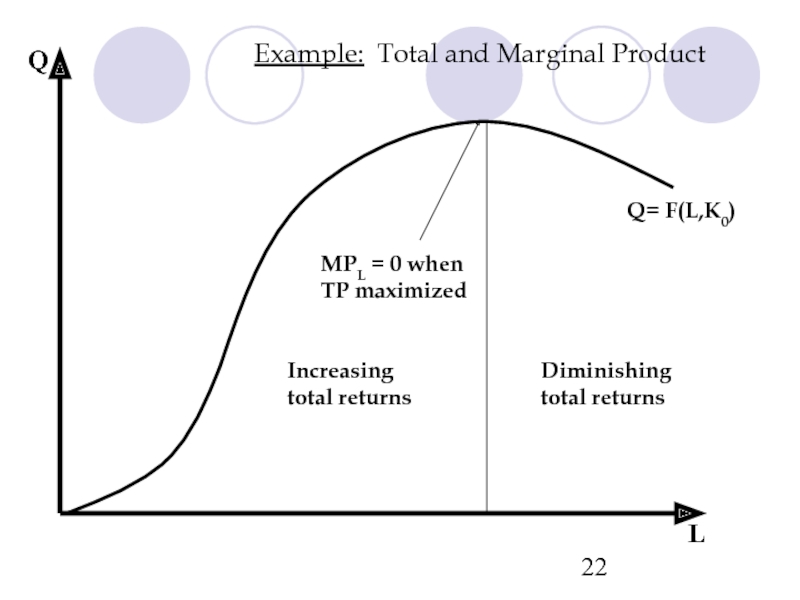
Слайд 22Q
L
MPL = 0 when
TP maximized
Q= F(L,K0)
Example: Total and Marginal Product
Diminishing total
Increasing total returns
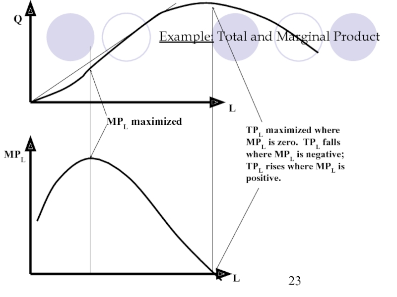
Слайд 23Example: Total and Marginal Product
L
MPL
Q
L
MPL maximized
TPL maximized where
MPL is zero. TPL
where MPL is negative;
TPL rises where MPL is
positive.
Слайд 24Marginal and Average Products
There is a systematic relationship between average product
This relationship holds for any comparison between any marginal magnitude with the average magnitude.
Слайд 25Marginal and Average Products
When marginal product is greater than average product,
E.g., if MPL > APL , APL increases in L.
When marginal product is less than average product, average product is decreasing.
E.g., if MPL < APL, APL decreases in L.
Слайд 28Isoquants
Definition: An isoquant is a representation of all the combinations of
Слайд 30L
Q = 10
Q = 20
All combinations of (L,K) along the
isoquant produce
0
Slope=dK/dL
K
Example: Isoquants
Слайд 31Isoquants
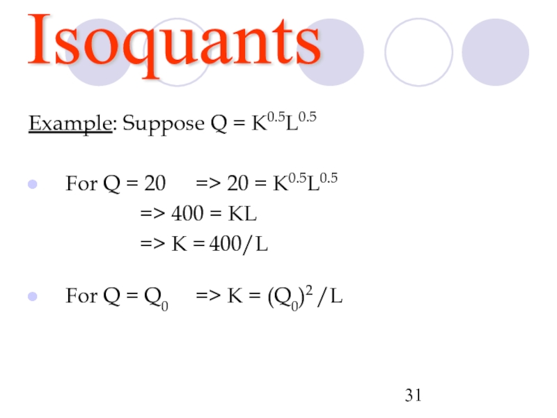
Example: Suppose Q = K0.5L0.5
For Q = 20 => 20 =
=> 400 = KL
=> K = 400/L
For Q = Q0 => K = (Q0)2 /L
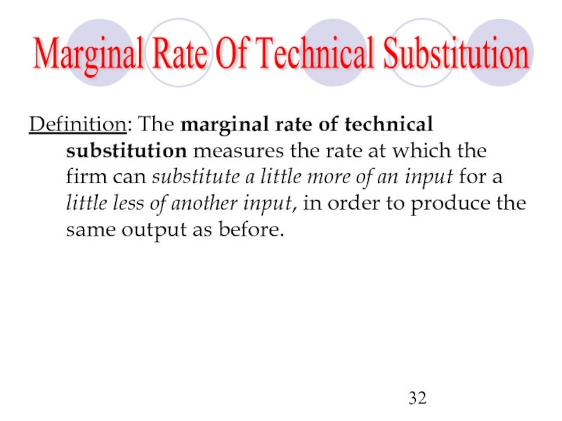
Слайд 32Definition: The marginal rate of technical substitution measures the rate at
Marginal Rate Of Technical Substitution
Слайд 33Marginal Rate Of Technical Substitution
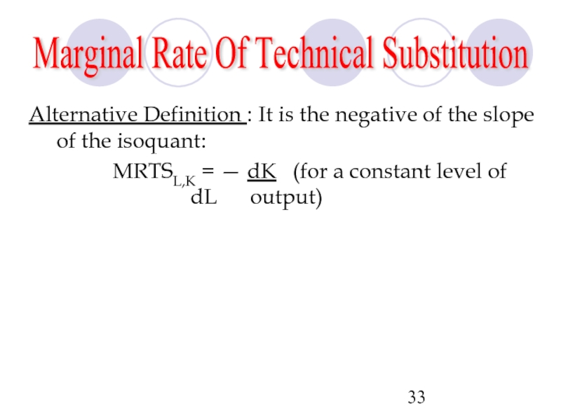
Alternative Definition : It is the
MRTSL,K = — dK (for a constant level of
dL output)
Слайд 34Marginal Product and the Marginal
Rate of Technical Substitution
We can
Using differentials, along a particular isoquant:
MPL . dL + MPK . dK = dQ = 0
Solving:
MPL = _ dK = MRTSL,K
MPK dL
Слайд 35Marginal Product and the Marginal
Rate of Technical Substitution
Notes:
If we
In other words, the marginal rate of technical substitution of labour for capital diminishes as the quantity of labour increases along an isoquant.
Слайд 36Marginal Product and the Marginal
Rate of Technical Substitution
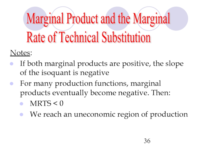
Notes:
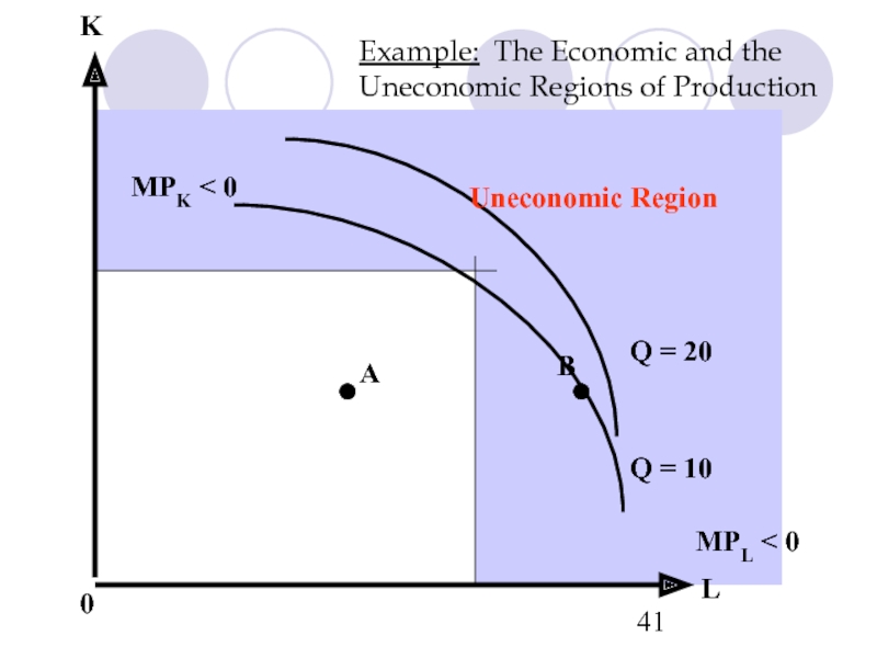
If both
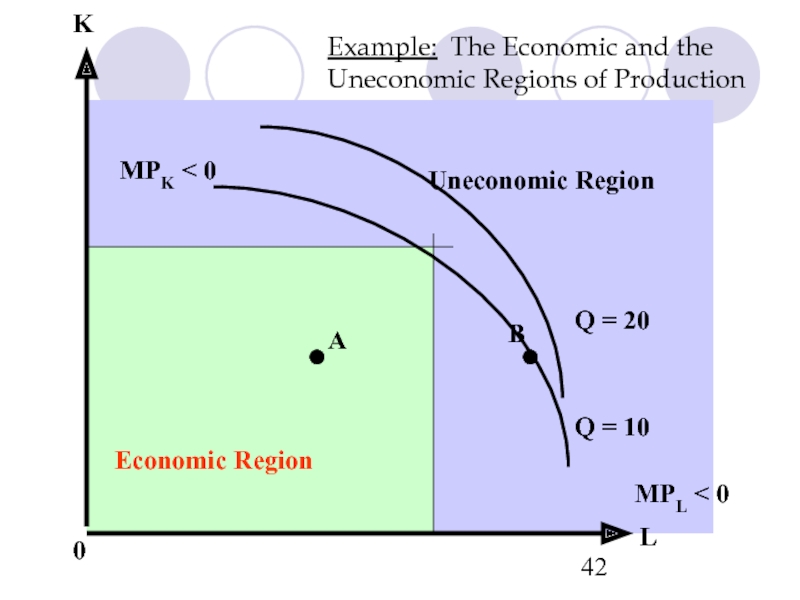
For many production functions, marginal products eventually become negative. Then:
MRTS < 0
We reach an uneconomic region of production
Слайд 40Example: The Economic and the Uneconomic Regions of Production
L
K
Q =
Q = 20
0
MPK < 0
MPL < 0
•
•
B
A
Слайд 41
Example: The Economic and the Uneconomic Regions of Production
L
K
Q =
Q = 20
0
MPK < 0
MPL < 0
•
•
B
A
Uneconomic Region
Слайд 42
Example: The Economic and the Uneconomic Regions of Production
L
K
Q =
Q = 20
0
MPK < 0
MPL < 0
•
•
B
A
Uneconomic Region
Economic Region
