- Главная
- Разное
- Дизайн
- Бизнес и предпринимательство
- Аналитика
- Образование
- Развлечения
- Красота и здоровье
- Финансы
- Государство
- Путешествия
- Спорт
- Недвижимость
- Армия
- Графика
- Культурология
- Еда и кулинария
- Лингвистика
- Английский язык
- Астрономия
- Алгебра
- Биология
- География
- Детские презентации
- Информатика
- История
- Литература
- Маркетинг
- Математика
- Медицина
- Менеджмент
- Музыка
- МХК
- Немецкий язык
- ОБЖ
- Обществознание
- Окружающий мир
- Педагогика
- Русский язык
- Технология
- Физика
- Философия
- Химия
- Шаблоны, картинки для презентаций
- Экология
- Экономика
- Юриспруденция
Financial econometrics презентация
Содержание
- 1. Financial econometrics
- 2. Financial Econometrics 2016 – Dr. Kashif
- 3. Quantitative Economic Analysis – 2016, Dr. Kashif
- 4. Financial Econometrics 2016 – Dr. Kashif
- 5. Financial Econometrics 2016 – Dr. Kashif
- 6. Financial Econometrics 2016 – Dr. Kashif
- 7. Financial Econometrics 2016 – Dr. Kashif
- 8. Financial Econometrics 2016 – Dr. Kashif
- 9. Financial Econometrics 2016 – Dr. Kashif
- 10. Financial Econometrics 2016 – Dr. Kashif
- 11. Financial Econometrics 2016 – Dr. Kashif
- 12. Financial Econometrics 2016 – Dr. Kashif
- 13. Financial Econometrics 2016 – Dr. Kashif
- 14. Financial Econometrics 2016 – Dr. Kashif
- 15. Financial Econometrics 2016 – Dr. Kashif
- 16. Financial Econometrics 2016 – Dr. Kashif
- 17. Financial Econometrics 2016 – Dr. Kashif
- 18. Financial Econometrics 2016 – Dr. Kashif
- 19. Financial Econometrics 2016 – Dr. Kashif
- 20. Financial Econometrics 2016 – Dr. Kashif
- 21. Financial Econometrics 2016 – Dr. Kashif
- 22. Financial Econometrics 2016 – Dr. Kashif
- 23. Financial Econometrics 2016 – Dr. Kashif
- 24. Financial Econometrics 2016 – Dr. Kashif
- 25. Financial Econometrics 2016 – Dr. Kashif
- 26. Financial Econometrics 2016 – Dr. Kashif
- 27. Financial Econometrics 2016 – Dr. Kashif
- 28. Financial Econometrics 2016 – Dr. Kashif
- 29. Financial Econometrics 2016 – Dr. Kashif
- 30. Financial Econometrics 2016 – Dr. Kashif
- 31. Financial Econometrics 2016 – Dr. Kashif
- 32. Financial Econometrics 2016 – Dr. Kashif
- 33. Financial Econometrics 2016 – Dr. Kashif
- 34. Financial Econometrics 2016 – Dr. Kashif
- 35. Financial Econometrics 2016 – Dr. Kashif
- 36. Financial Econometrics 2016 – Dr. Kashif
- 37. Financial Econometrics 2016 – Dr. Kashif
- 38. Financial Econometrics 2016 – Dr. Kashif
- 39. Home Assignment Vector Autoregressive Model: Run
- 40. Home Assignment ARMA FAMILY MODELS: Use
Слайд 1Financial Econometrics 2016 – Dr. Kashif Saleem (UOWD)
Financial Econometrics
Dr. Kashif
Associate Professor (Finance)
University of Wollongong in Dubai
Слайд 2Financial Econometrics 2016 – Dr. Kashif Saleem (UOWD)
Univariate time series
Univariate time series modelling
Moving average processes
Autoregressive processes
ARMA processes
ARIMA process
Exponential Smoothing
Forecasting in Econometrics
Vector Autoregressive Models
Слайд 3Quantitative Economic Analysis – 2016, Dr. Kashif Saleem (UOWD)
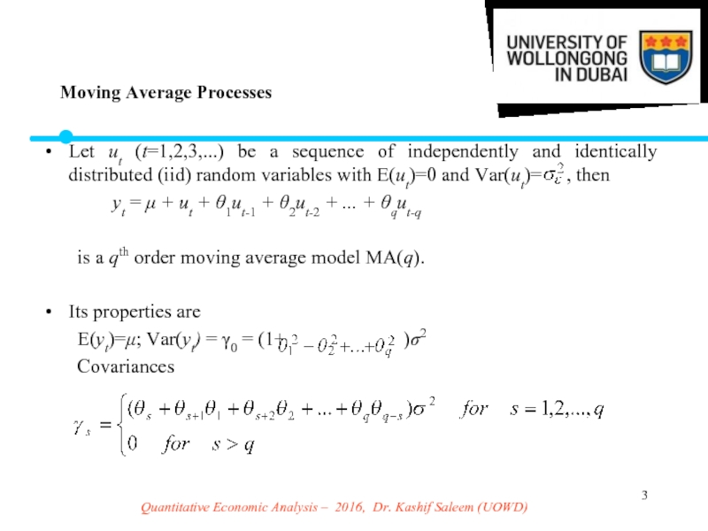
Let ut (t=1,2,3,...)
yt = μ + ut + θ1ut-1 + θ2ut-2 + ... + θqut-q
is a qth order moving average model MA(q).
Its properties are
E(yt)=μ; Var(yt) = γ0 = (1+ )σ2
Covariances
Moving Average Processes
Слайд 4Financial Econometrics 2016 – Dr. Kashif Saleem (UOWD)
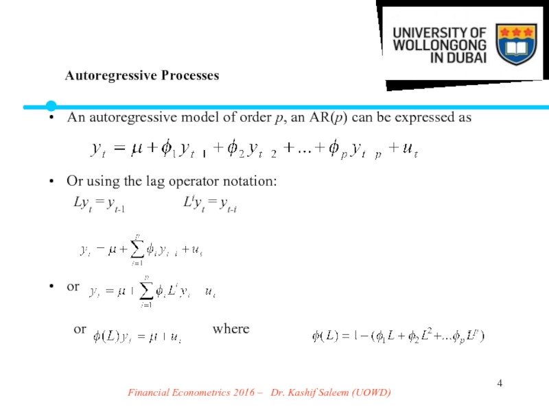
An autoregressive model
Or using the lag operator notation:
Lyt = yt-1 Liyt = yt-i
or
or where .
Autoregressive Processes
Слайд 5Financial Econometrics 2016 – Dr. Kashif Saleem (UOWD)
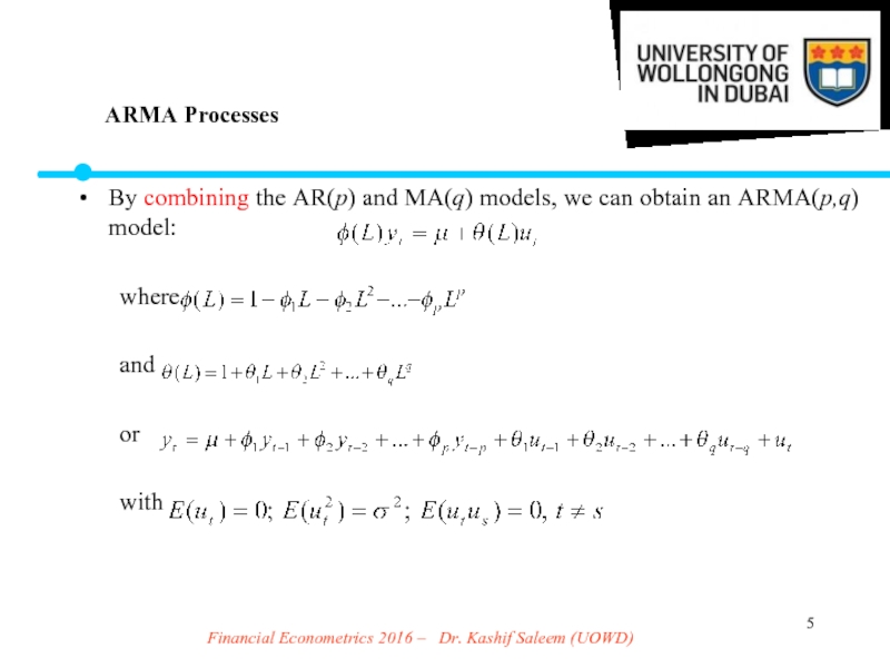
By combining the
where
and
or
with
ARMA Processes
Слайд 6Financial Econometrics 2016 – Dr. Kashif Saleem (UOWD)
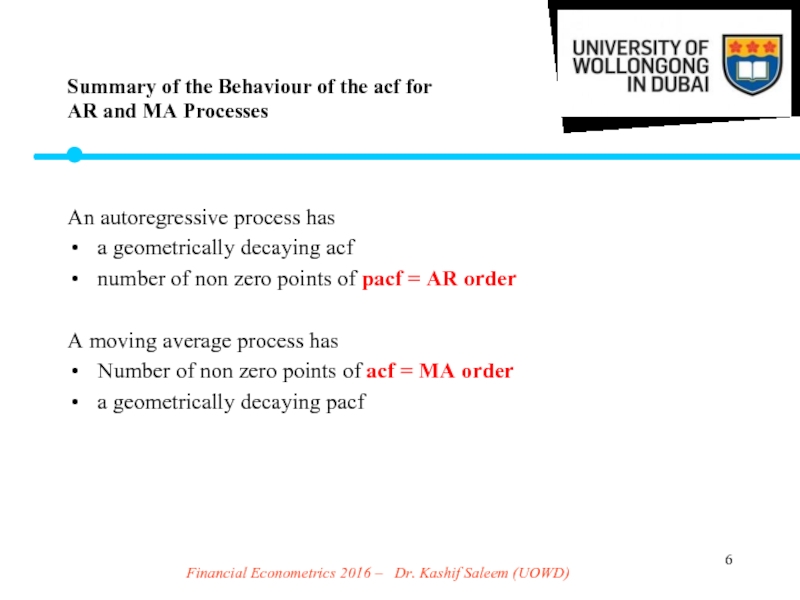
An autoregressive process
a geometrically decaying acf
number of non zero points of pacf = AR order
A moving average process has
Number of non zero points of acf = MA order
a geometrically decaying pacf
Summary of the Behaviour of the acf for
AR and MA Processes
Слайд 7Financial Econometrics 2016 – Dr. Kashif Saleem (UOWD)
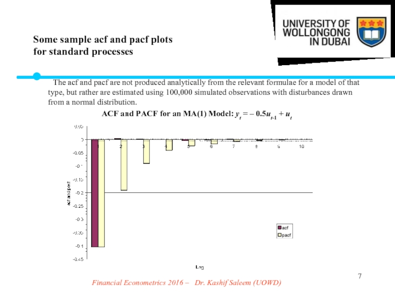
The acf and
ACF and PACF for an MA(1) Model: yt = – 0.5ut-1 + ut
Some sample acf and pacf plots
for standard processes
Слайд 8Financial Econometrics 2016 – Dr. Kashif Saleem (UOWD)
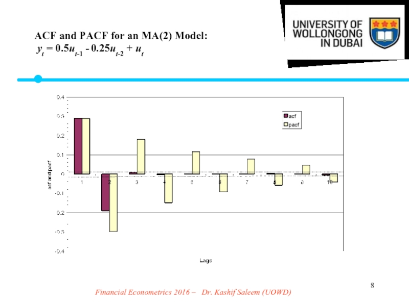
ACF and PACF
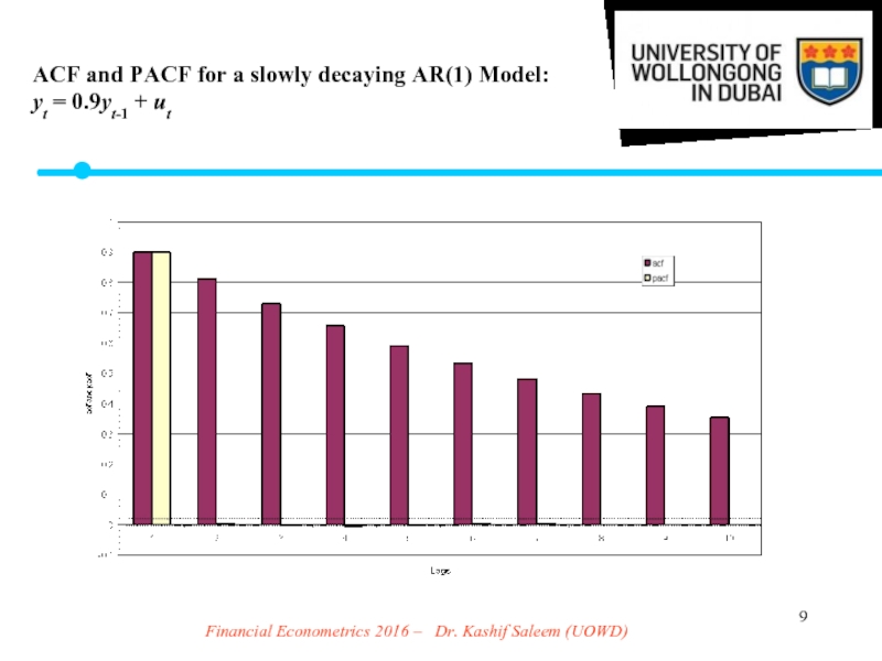
Слайд 9Financial Econometrics 2016 – Dr. Kashif Saleem (UOWD)
ACF and PACF
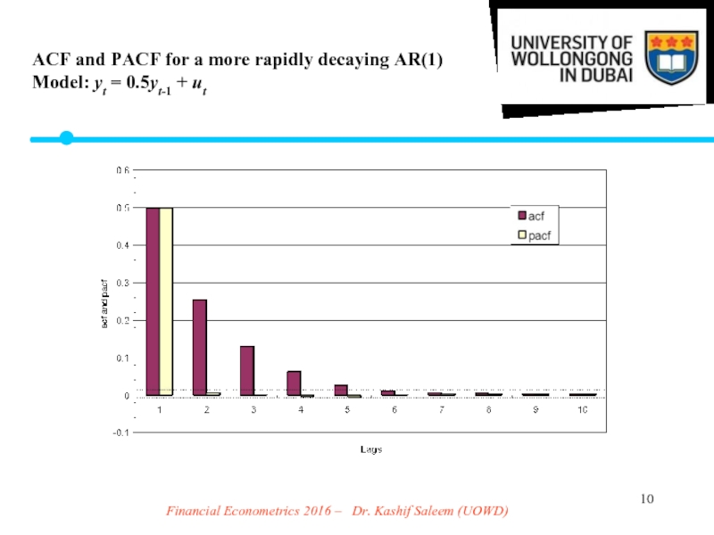
Слайд 10Financial Econometrics 2016 – Dr. Kashif Saleem (UOWD)
ACF and PACF
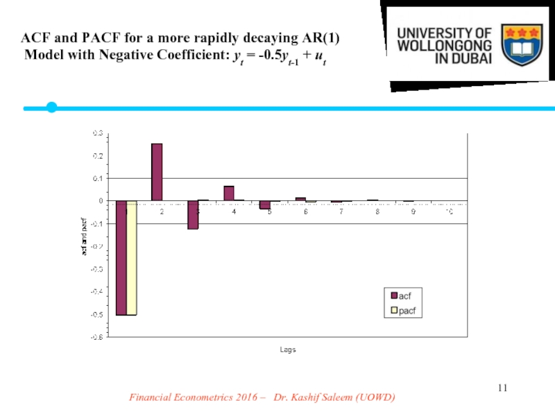
Слайд 11Financial Econometrics 2016 – Dr. Kashif Saleem (UOWD)
ACF and PACF
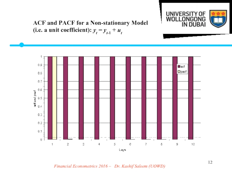
Слайд 12Financial Econometrics 2016 – Dr. Kashif Saleem (UOWD)
ACF and PACF
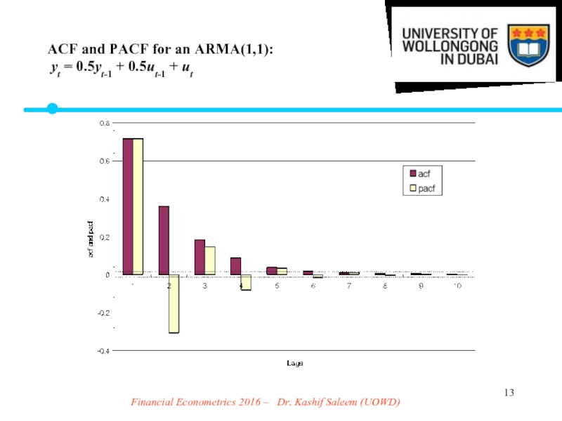
Слайд 13Financial Econometrics 2016 – Dr. Kashif Saleem (UOWD)
ACF and PACF
Слайд 14Financial Econometrics 2016 – Dr. Kashif Saleem (UOWD)
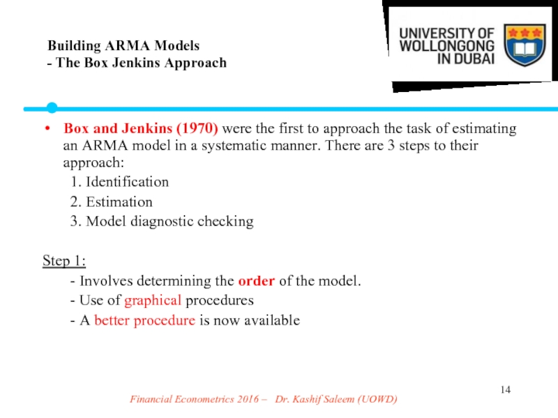
Box and Jenkins
1. Identification
2. Estimation
3. Model diagnostic checking
Step 1:
- Involves determining the order of the model.
- Use of graphical procedures
- A better procedure is now available
Building ARMA Models
- The Box Jenkins Approach
Слайд 15Financial Econometrics 2016 – Dr. Kashif Saleem (UOWD)
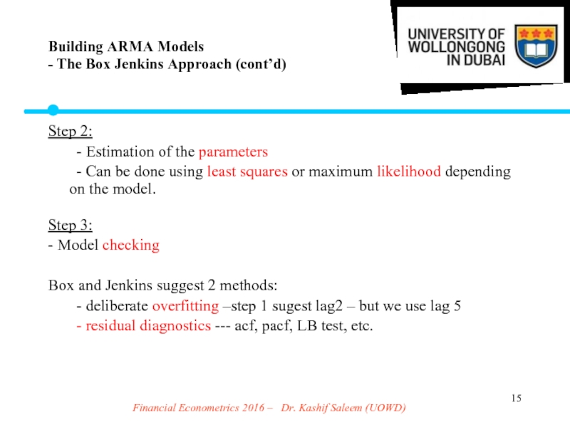
Step 2:
- Estimation
- Can be done using least squares or maximum likelihood depending on the model.
Step 3:
- Model checking
Box and Jenkins suggest 2 methods:
- deliberate overfitting –step 1 sugest lag2 – but we use lag 5
- residual diagnostics --- acf, pacf, LB test, etc.
Building ARMA Models
- The Box Jenkins Approach (cont’d)
Слайд 16Financial Econometrics 2016 – Dr. Kashif Saleem (UOWD)
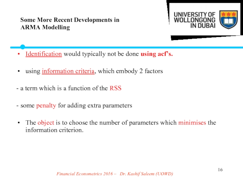
Identification would typically
using information criteria, which embody 2 factors
- a term which is a function of the RSS
- some penalty for adding extra parameters
The object is to choose the number of parameters which minimises the information criterion.
Some More Recent Developments in
ARMA Modelling
Слайд 17Financial Econometrics 2016 – Dr. Kashif Saleem (UOWD)
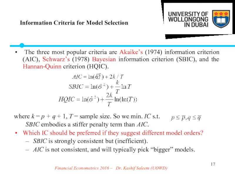
The three most
where k = p + q + 1, T = sample size. So we min. IC s.t.
SBIC embodies a stiffer penalty term than AIC.
Which IC should be preferred if they suggest different model orders?
SBIC is strongly consistent but (inefficient).
AIC is not consistent, and will typically pick “bigger” models.
Information Criteria for Model Selection
Слайд 18Financial Econometrics 2016 – Dr. Kashif Saleem (UOWD)
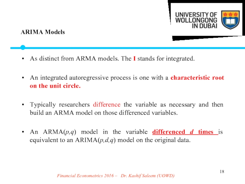
As distinct from
An integrated autoregressive process is one with a characteristic root on the unit circle.
Typically researchers difference the variable as necessary and then build an ARMA model on those differenced variables.
An ARMA(p,q) model in the variable differenced d times is equivalent to an ARIMA(p,d,q) model on the original data.
ARIMA Models
Слайд 19Financial Econometrics 2016 – Dr. Kashif Saleem (UOWD)
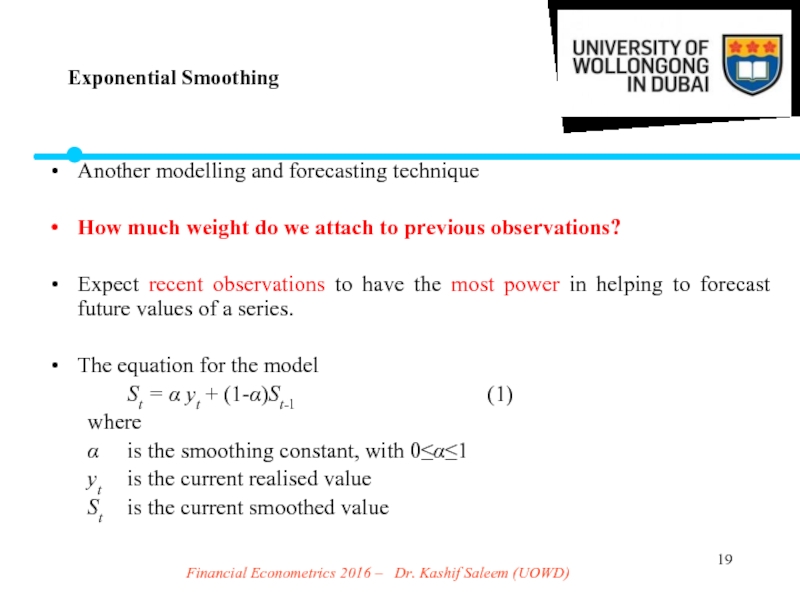
Another modelling and
How much weight do we attach to previous observations?
Expect recent observations to have the most power in helping to forecast future values of a series.
The equation for the model
St = α yt + (1-α)St-1 (1)
where
α is the smoothing constant, with 0≤α≤1
yt is the current realised value
St is the current smoothed value
Exponential Smoothing
Слайд 20Financial Econometrics 2016 – Dr. Kashif Saleem (UOWD)
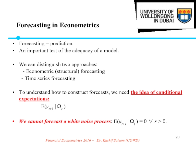
Forecasting = prediction.
An
We can distinguish two approaches:
- Econometric (structural) forecasting
- Time series forecasting
To understand how to construct forecasts, we need the idea of conditional expectations:
E(yt+1 | Ωt )
We cannot forecast a white noise process: E(ut+s | Ωt ) = 0 ∀ s > 0.
Forecasting in Econometrics
Слайд 21Financial Econometrics 2016 – Dr. Kashif Saleem (UOWD)
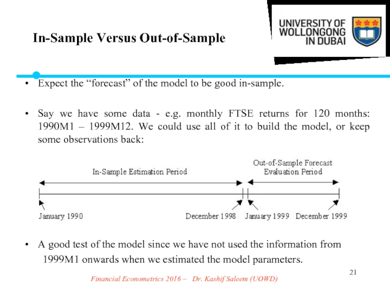
Expect the “forecast”
Say we have some data - e.g. monthly FTSE returns for 120 months: 1990M1 – 1999M12. We could use all of it to build the model, or keep some observations back:
A good test of the model since we have not used the information from
1999M1 onwards when we estimated the model parameters.
In-Sample Versus Out-of-Sample
Слайд 22Financial Econometrics 2016 – Dr. Kashif Saleem (UOWD)
Models for Forecasting
Time Series Models
The current value of a series, yt, is modelled as a function only of its previous values and the current value of an error term (and possibly previous values of the error term).
Models include:
simple unweighted averages
exponentially weighted averages
ARIMA models
Non-linear models – e.g. threshold models, GARCH, bilinear models, etc.
Слайд 23Financial Econometrics 2016 – Dr. Kashif Saleem (UOWD)
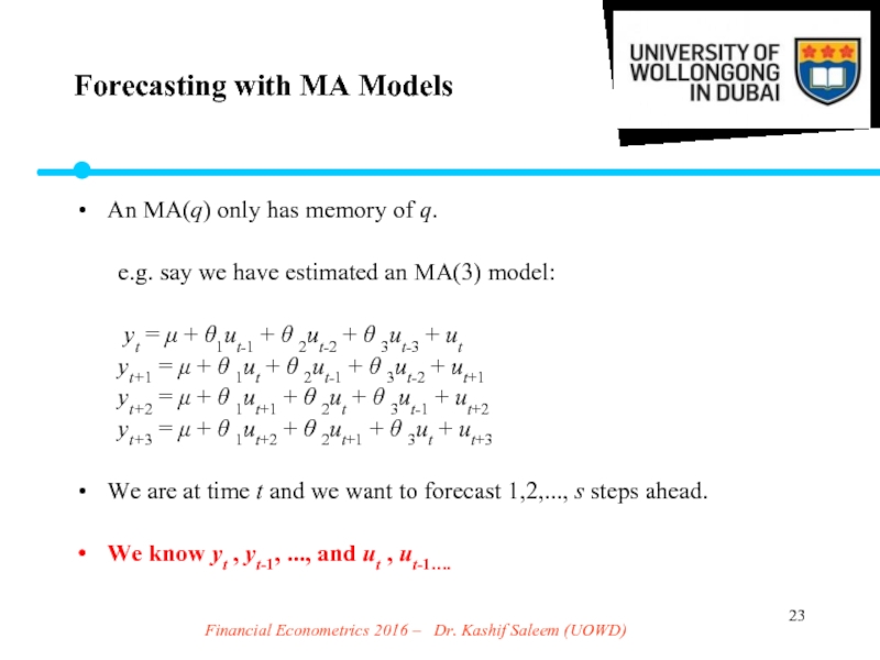
An MA(q) only
e.g. say we have estimated an MA(3) model:
yt = μ + θ1ut-1 + θ 2ut-2 + θ 3ut-3 + ut
yt+1 = μ + θ 1ut + θ 2ut-1 + θ 3ut-2 + ut+1
yt+2 = μ + θ 1ut+1 + θ 2ut + θ 3ut-1 + ut+2
yt+3 = μ + θ 1ut+2 + θ 2ut+1 + θ 3ut + ut+3
We are at time t and we want to forecast 1,2,..., s steps ahead.
We know yt , yt-1, ..., and ut , ut-1….
Forecasting with MA Models
Слайд 24Financial Econometrics 2016 – Dr. Kashif Saleem (UOWD)
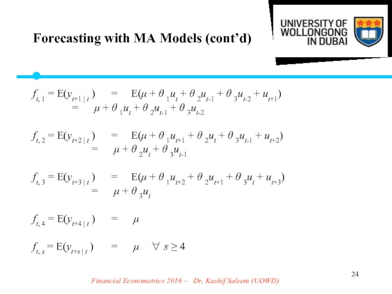
ft, 1 =
= μ + θ 1ut + θ 2ut-1 + θ 3ut-2
ft, 2 = E(yt+2 | t ) = E(μ + θ 1ut+1 + θ 2ut + θ 3ut-1 + ut+2)
= μ + θ 2ut + θ 3ut-1
ft, 3 = E(yt+3 | t ) = E(μ + θ 1ut+2 + θ 2ut+1 + θ 3ut + ut+3)
= μ + θ 3ut
ft, 4 = E(yt+4 | t ) = μ
ft, s = E(yt+s | t ) = μ ∀ s ≥ 4
Forecasting with MA Models (cont’d)
Слайд 25Financial Econometrics 2016 – Dr. Kashif Saleem (UOWD)
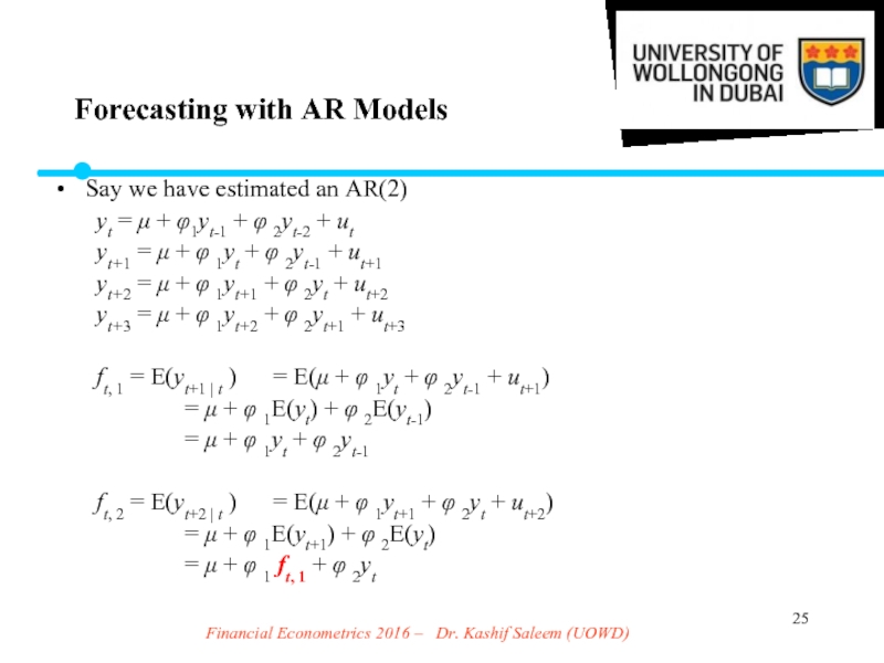
Say we have
yt = μ + φ1yt-1 + φ 2yt-2 + ut
yt+1 = μ + φ 1yt + φ 2yt-1 + ut+1
yt+2 = μ + φ 1yt+1 + φ 2yt + ut+2
yt+3 = μ + φ 1yt+2 + φ 2yt+1 + ut+3
ft, 1 = E(yt+1 | t ) = E(μ + φ 1yt + φ 2yt-1 + ut+1)
= μ + φ 1E(yt) + φ 2E(yt-1)
= μ + φ 1yt + φ 2yt-1
ft, 2 = E(yt+2 | t ) = E(μ + φ 1yt+1 + φ 2yt + ut+2)
= μ + φ 1E(yt+1) + φ 2E(yt)
= μ + φ 1 ft, 1 + φ 2yt
Forecasting with AR Models
Слайд 26Financial Econometrics 2016 – Dr. Kashif Saleem (UOWD)
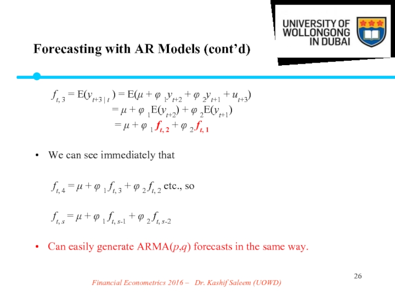
ft, 3 =
= μ + φ 1E(yt+2) + φ 2E(yt+1)
= μ + φ 1 ft, 2 + φ 2 ft, 1
We can see immediately that
ft, 4 = μ + φ 1 ft, 3 + φ 2 ft, 2 etc., so
ft, s = μ + φ 1 ft, s-1 + φ 2 ft, s-2
Can easily generate ARMA(p,q) forecasts in the same way.
Forecasting with AR Models (cont’d)
Слайд 27Financial Econometrics 2016 – Dr. Kashif Saleem (UOWD)
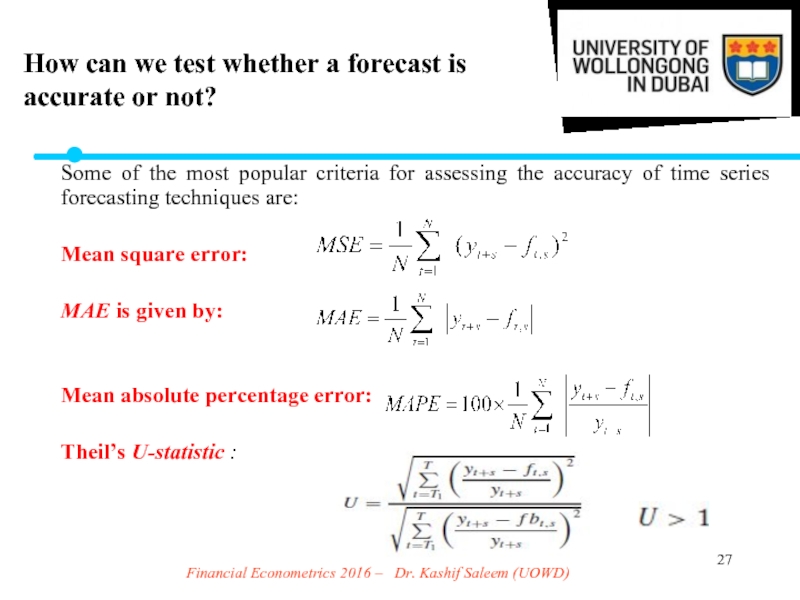
Some of the
Mean square error:
MAE is given by:
Mean absolute percentage error:
Theil’s U-statistic :
How can we test whether a forecast is accurate or not?
Слайд 28Financial Econometrics 2016 – Dr. Kashif Saleem (UOWD)
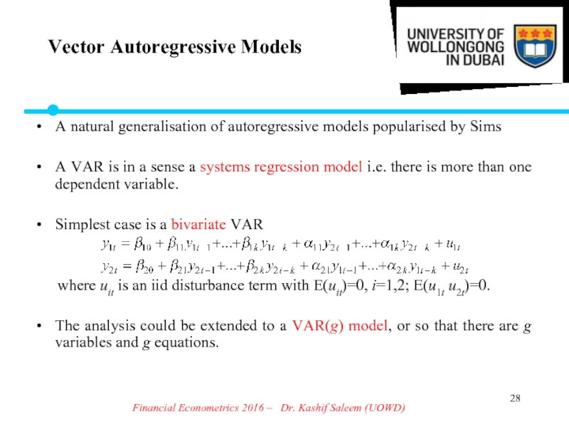
A natural generalisation
A VAR is in a sense a systems regression model i.e. there is more than one dependent variable.
Simplest case is a bivariate VAR
where uit is an iid disturbance term with E(uit)=0, i=1,2; E(u1t u2t)=0.
The analysis could be extended to a VAR(g) model, or so that there are g variables and g equations.
Vector Autoregressive Models
Слайд 29Financial Econometrics 2016 – Dr. Kashif Saleem (UOWD)
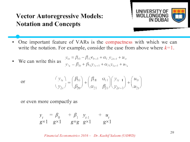
One important feature
We can write this as
or
or even more compactly as
yt = β0 + β1 yt-1 + ut
g×1 g×1 g×g g×1 g×1
Vector Autoregressive Models:
Notation and Concepts
Слайд 30Financial Econometrics 2016 – Dr. Kashif Saleem (UOWD)
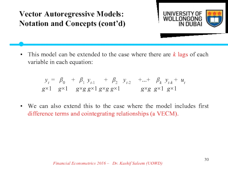
This model can
yt = β0 + β1 yt-1 + β2 yt-2 +...+ βk yt-k + ut
g×1 g×1 g×g g×1 g×g g×1 g×g g×1 g×1
We can also extend this to the case where the model includes first difference terms and cointegrating relationships (a VECM).
Vector Autoregressive Models:
Notation and Concepts (cont’d)
Слайд 31Financial Econometrics 2016 – Dr. Kashif Saleem (UOWD)
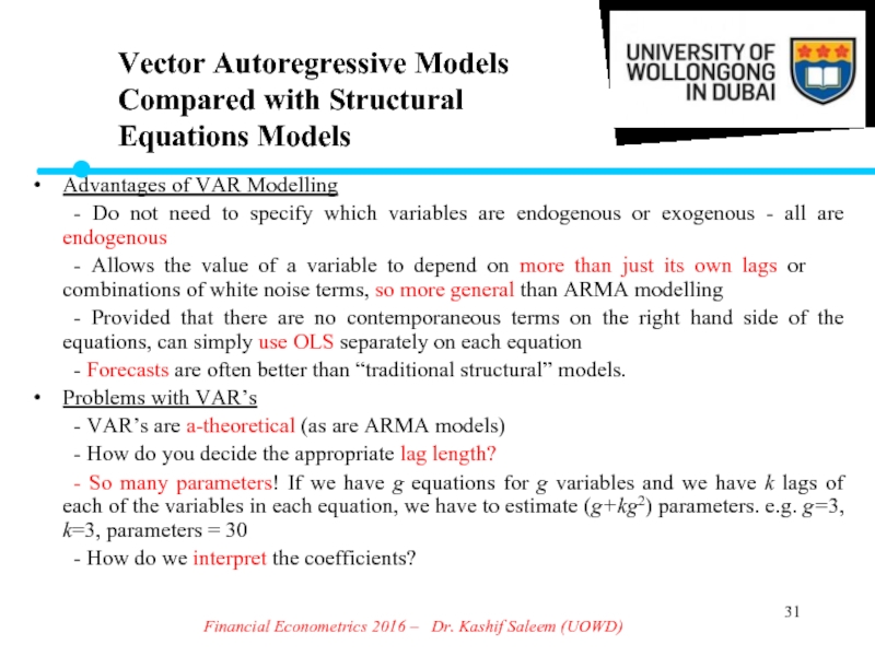
Advantages of VAR
- Do not need to specify which variables are endogenous or exogenous - all are endogenous
- Allows the value of a variable to depend on more than just its own lags or combinations of white noise terms, so more general than ARMA modelling
- Provided that there are no contemporaneous terms on the right hand side of the equations, can simply use OLS separately on each equation
- Forecasts are often better than “traditional structural” models.
Problems with VAR’s
- VAR’s are a-theoretical (as are ARMA models)
- How do you decide the appropriate lag length?
- So many parameters! If we have g equations for g variables and we have k lags of each of the variables in each equation, we have to estimate (g+kg2) parameters. e.g. g=3, k=3, parameters = 30
- How do we interpret the coefficients?
Vector Autoregressive Models Compared with Structural Equations Models
Слайд 32Financial Econometrics 2016 – Dr. Kashif Saleem (UOWD)
Choosing the Optimal
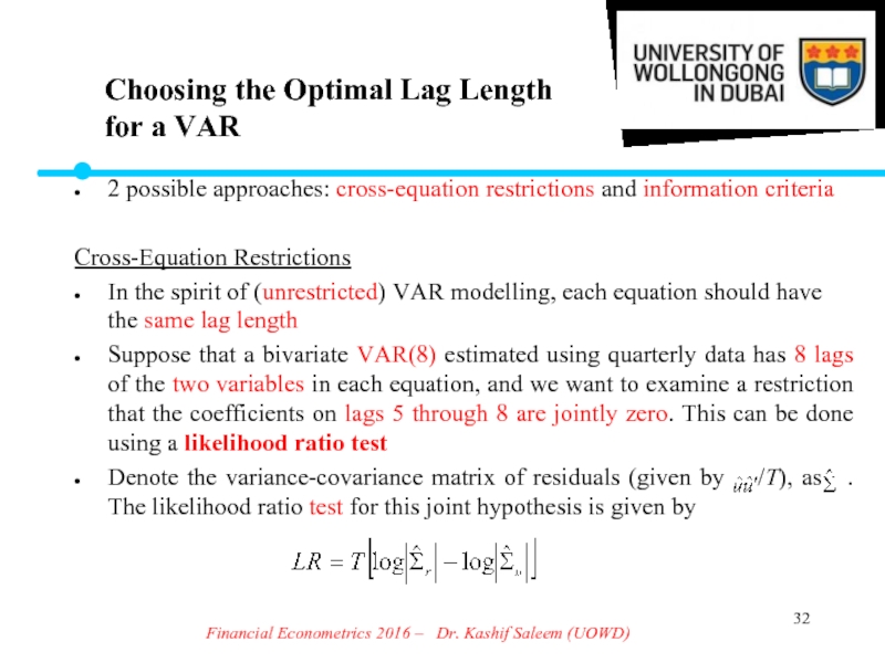
2 possible approaches: cross-equation restrictions and information criteria
Cross-Equation Restrictions
In the spirit of (unrestricted) VAR modelling, each equation should have the same lag length
Suppose that a bivariate VAR(8) estimated using quarterly data has 8 lags of the two variables in each equation, and we want to examine a restriction that the coefficients on lags 5 through 8 are jointly zero. This can be done using a likelihood ratio test
Denote the variance-covariance matrix of residuals (given by /T), as . The likelihood ratio test for this joint hypothesis is given by
Слайд 33Financial Econometrics 2016 – Dr. Kashif Saleem (UOWD)
Choosing the Optimal
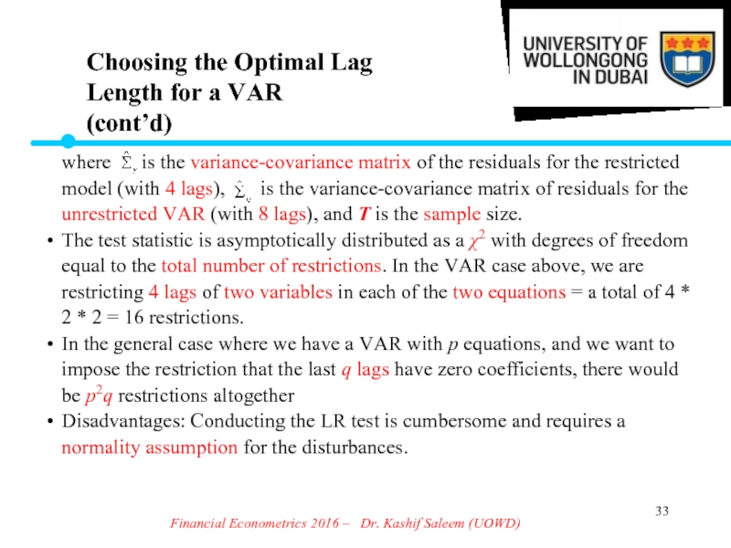
where is the variance-covariance matrix of the residuals for the restricted
model (with 4 lags), is the variance-covariance matrix of residuals for the
unrestricted VAR (with 8 lags), and T is the sample size.
The test statistic is asymptotically distributed as a χ2 with degrees of freedom
equal to the total number of restrictions. In the VAR case above, we are
restricting 4 lags of two variables in each of the two equations = a total of 4 *
2 * 2 = 16 restrictions.
In the general case where we have a VAR with p equations, and we want to
impose the restriction that the last q lags have zero coefficients, there would
be p2q restrictions altogether
Disadvantages: Conducting the LR test is cumbersome and requires a
normality assumption for the disturbances.
Слайд 34Financial Econometrics 2016 – Dr. Kashif Saleem (UOWD)
Information Criteria for
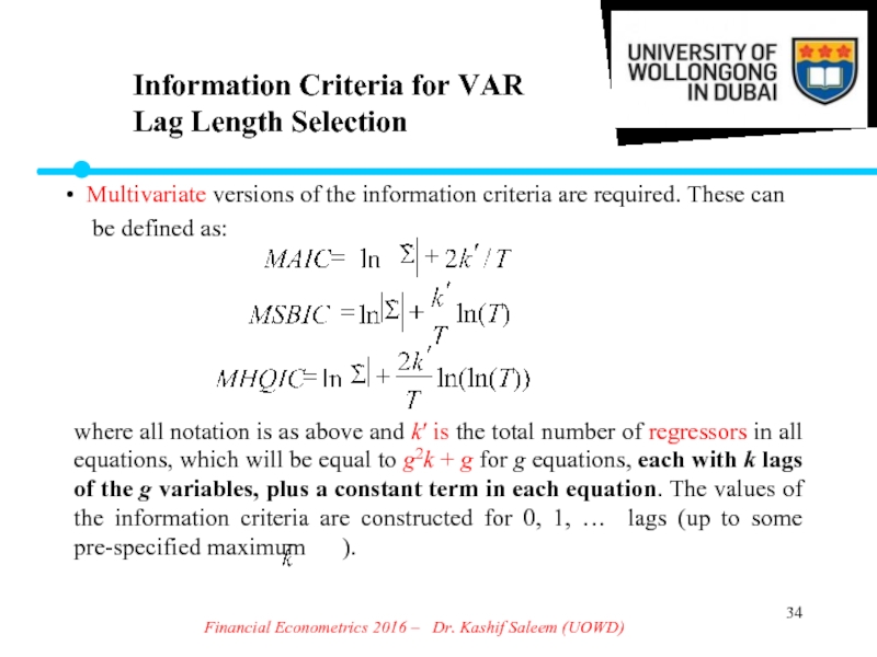
Multivariate versions of the information criteria are required. These can
be defined as:
where all notation is as above and k′ is the total number of regressors in all equations, which will be equal to g2k + g for g equations, each with k lags of the g variables, plus a constant term in each equation. The values of the information criteria are constructed for 0, 1, … lags (up to some pre-specified maximum ).
Слайд 35Financial Econometrics 2016 – Dr. Kashif Saleem (UOWD)
Block Significance and
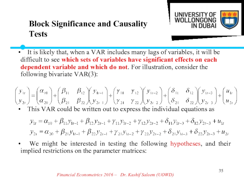
It is likely that, when a VAR includes many lags of variables, it will be difficult to see which sets of variables have significant effects on each dependent variable and which do not. For illustration, consider the following bivariate VAR(3):
This VAR could be written out to express the individual equations as
We might be interested in testing the following hypotheses, and their implied restrictions on the parameter matrices:
Слайд 36Financial Econometrics 2016 – Dr. Kashif Saleem (UOWD)
Block Significance and
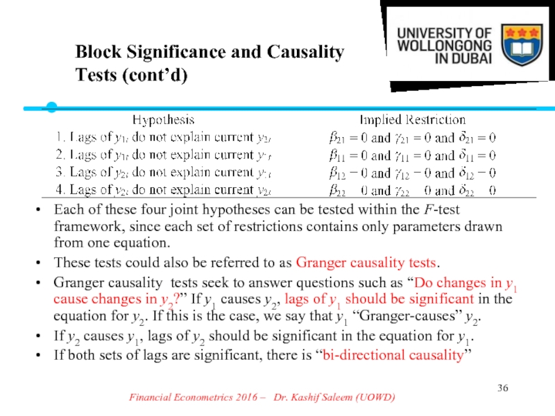
Each of these four joint hypotheses can be tested within the F-test framework, since each set of restrictions contains only parameters drawn from one equation.
These tests could also be referred to as Granger causality tests.
Granger causality tests seek to answer questions such as “Do changes in y1 cause changes in y2?” If y1 causes y2, lags of y1 should be significant in the equation for y2. If this is the case, we say that y1 “Granger-causes” y2.
If y2 causes y1, lags of y2 should be significant in the equation for y1.
If both sets of lags are significant, there is “bi-directional causality”
Слайд 37Financial Econometrics 2016 – Dr. Kashif Saleem (UOWD)
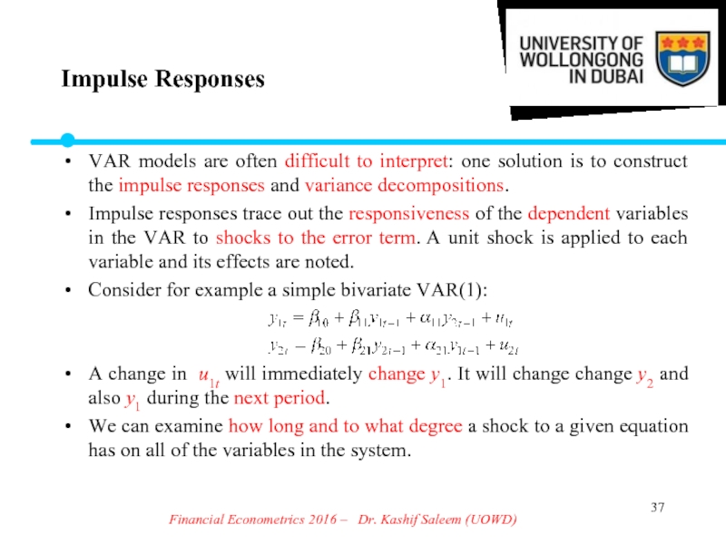
Impulse Responses
VAR models
Impulse responses trace out the responsiveness of the dependent variables in the VAR to shocks to the error term. A unit shock is applied to each variable and its effects are noted.
Consider for example a simple bivariate VAR(1):
A change in u1t will immediately change y1. It will change change y2 and also y1 during the next period.
We can examine how long and to what degree a shock to a given equation has on all of the variables in the system.
Слайд 38Financial Econometrics 2016 – Dr. Kashif Saleem (UOWD)
Variance Decompositions
Variance
This is done by determining how much of the s-step ahead forecast error variance for each variable is explained innovations to each explanatory variable (s = 1,2,…).
The variance decomposition gives information about the relative importance of each shock to the variables in the VAR.
Слайд 39Home Assignment
Vector Autoregressive Model:
Run a VAR (3) model by using
Conduct Block Significance and Causality Tests on your model
Present graphically Impulse Responses
Present graphically Variance Decompositions
Interpret your results
Financial Econometrics 2016 – Dr. Kashif Saleem (UOWD)
Слайд 40Home Assignment
ARMA FAMILY MODELS:
Use MICEX data to run the following models
MA (5)
AR (5)
ARMA (5,5)
ARMA (P,Q) – Based on the AIC Code
Interpret your results
Financial Econometrics 2016 – Dr. Kashif Saleem (UOWD)
