- Главная
- Разное
- Дизайн
- Бизнес и предпринимательство
- Аналитика
- Образование
- Развлечения
- Красота и здоровье
- Финансы
- Государство
- Путешествия
- Спорт
- Недвижимость
- Армия
- Графика
- Культурология
- Еда и кулинария
- Лингвистика
- Английский язык
- Астрономия
- Алгебра
- Биология
- География
- Детские презентации
- Информатика
- История
- Литература
- Маркетинг
- Математика
- Медицина
- Менеджмент
- Музыка
- МХК
- Немецкий язык
- ОБЖ
- Обществознание
- Окружающий мир
- Педагогика
- Русский язык
- Технология
- Физика
- Философия
- Химия
- Шаблоны, картинки для презентаций
- Экология
- Экономика
- Юриспруденция
Factor Models: Announcements, Surprises, and Expected Returns презентация
Содержание
- 1. Factor Models: Announcements, Surprises, and Expected Returns
- 2. 11.1 Factor Models: Announcements, Surprises, and
- 3. 11.1 Factor Models: Announcements, Surprises, and Expected
- 4. 11.1 Factor Models: Announcements, Surprises, and
- 5. 11.2 Risk: Systematic and Unsystematic A systematic
- 6. 11.2 Risk: Systematic and Unsystematic
- 7. 11.2 Risk: Systematic and Unsystematic Systematic risk
- 8. 11.3 Systematic Risk and Betas The beta
- 9. 11.3 Systematic Risk and Betas For example,
- 10. Systematic Risk and Betas: Example Suppose we
- 11. Systematic Risk and Betas: Example We must
- 12. Systematic Risk and Betas: Example If it
- 13. Systematic Risk and Betas: Example If it
- 14. Systematic Risk and Betas: Example Finally, if
- 15. 11.4 Portfolios and Factor Models Now let
- 16. Relationship Between the Return on
- 17. Relationship Between the Return on
- 18. Relationship Between the Return on
- 19. Portfolios and Diversification We know that the
- 20. Portfolios and Diversification The return on any
- 21. Portfolios and Diversification So the return on
- 22. 11.5 Betas and Expected Returns The return
- 23. Relationship Between β & Expected Return The
- 24. Relationship Between β & Expected Return
- 25. 11.6 The Capital Asset Pricing Model
- 26. Multi-factor APT Example: A Canadian study (Otuteye,
- 27. 11.7 Empirical Approaches to Asset Pricing Both
- 28. 11.8 Summary and Conclusions The APT assumes
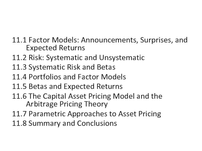
Слайд 111.1 Factor Models: Announcements, Surprises, and Expected Returns
11.2 Risk: Systematic and
11.3 Systematic Risk and Betas
11.4 Portfolios and Factor Models
11.5 Betas and Expected Returns
11.6 The Capital Asset Pricing Model and the Arbitrage Pricing Theory
11.7 Parametric Approaches to Asset Pricing
11.8 Summary and Conclusions
Слайд 2
11.1 Factor Models: Announcements, Surprises, and Expected Returns
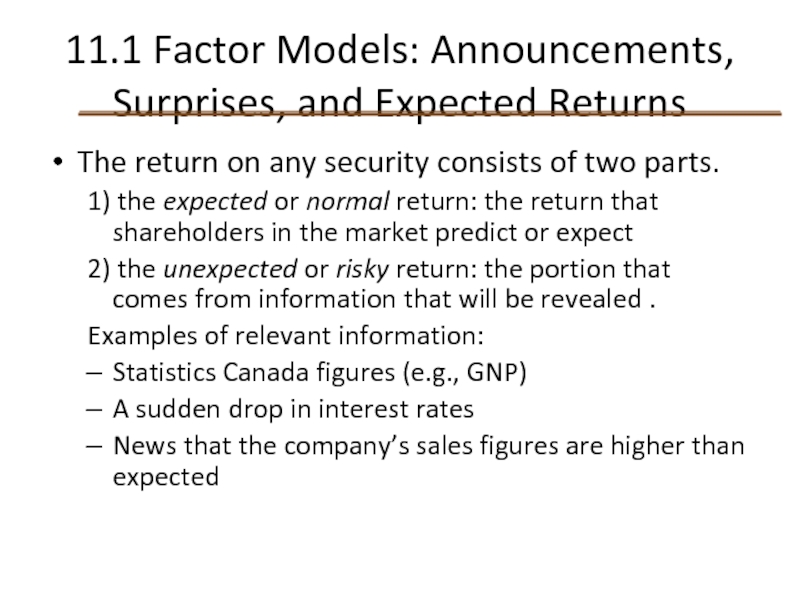
The return on any
1) the expected or normal return: the return that shareholders in the market predict or expect
2) the unexpected or risky return: the portion that comes from information that will be revealed .
Examples of relevant information:
Statistics Canada figures (e.g., GNP)
A sudden drop in interest rates
News that the company’s sales figures are higher than expected
Слайд 311.1 Factor Models: Announcements, Surprises, and Expected Returns
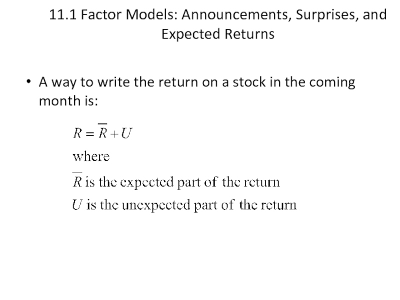
A way to write
Слайд 4
11.1 Factor Models: Announcements, Surprises, and Expected Returns
Any announcement can be
Announcement = Expected part + Surprise.
The expected part of any announcement is part of the information the market uses to form the expectation, R of the return on the stock.
The surprise is the news that influences the unanticipated return on the stock, U.
Слайд 511.2 Risk: Systematic and Unsystematic
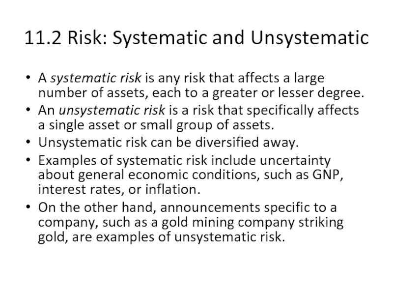
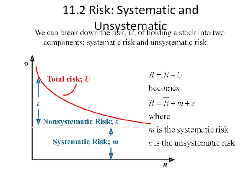
A systematic risk is any risk that
An unsystematic risk is a risk that specifically affects a single asset or small group of assets.
Unsystematic risk can be diversified away.
Examples of systematic risk include uncertainty about general economic conditions, such as GNP, interest rates, or inflation.
On the other hand, announcements specific to a company, such as a gold mining company striking gold, are examples of unsystematic risk.
Слайд 6
11.2 Risk: Systematic and Unsystematic
Systematic Risk; m
Nonsystematic Risk; ε
n
σ
Total risk;
We can break down the risk, U, of holding a stock into two components: systematic risk and unsystematic risk:
Слайд 711.2 Risk: Systematic and Unsystematic
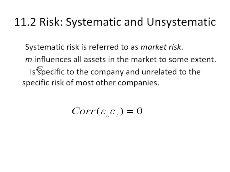
Systematic risk is referred to as market
m influences all assets in the market to some extent.
Is specific to the company and unrelated to the specific risk of most other companies.
Слайд 811.3 Systematic Risk and Betas
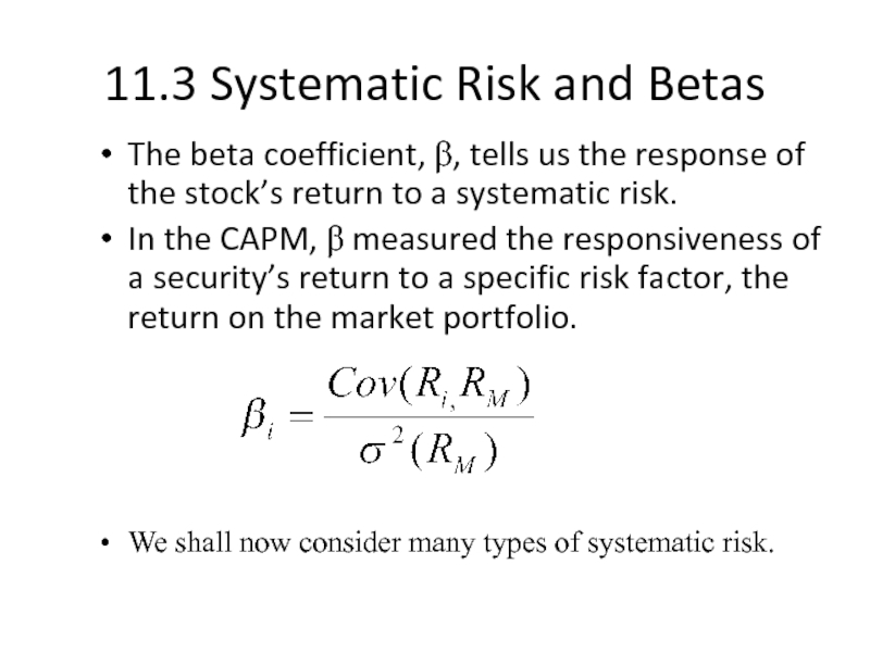
The beta coefficient, β, tells us the
In the CAPM, β measured the responsiveness of a security’s return to a specific risk factor, the return on the market portfolio.
We shall now consider many types of systematic risk.
Слайд 911.3 Systematic Risk and Betas
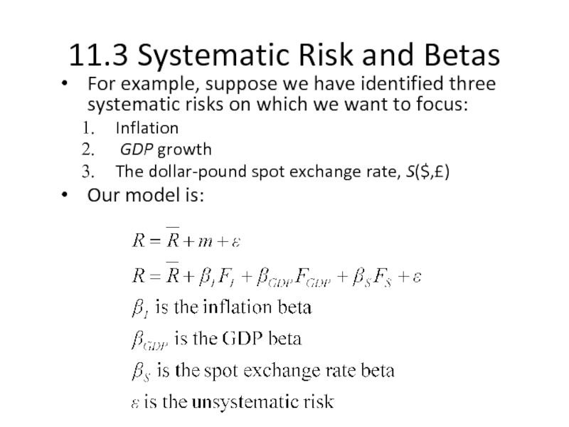
For example, suppose we have identified three
Inflation
GDP growth
The dollar-pound spot exchange rate, S($,£)
Our model is:
Слайд 10Systematic Risk and Betas: Example
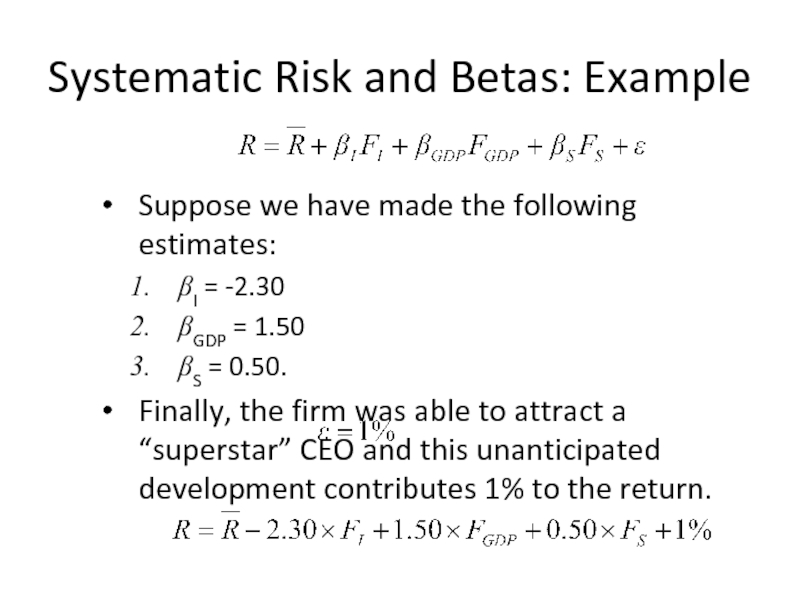
Suppose we have made the following estimates:
βI
βGDP = 1.50
βS = 0.50.
Finally, the firm was able to attract a “superstar” CEO and this unanticipated development contributes 1% to the return.
Слайд 11Systematic Risk and Betas: Example
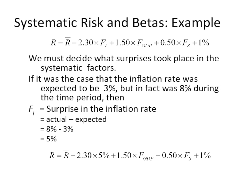
We must decide what surprises took place
If it was the case that the inflation rate was expected to be 3%, but in fact was 8% during the time period, then
FI = Surprise in the inflation rate
= actual – expected
= 8% - 3%
= 5%
Слайд 12Systematic Risk and Betas: Example
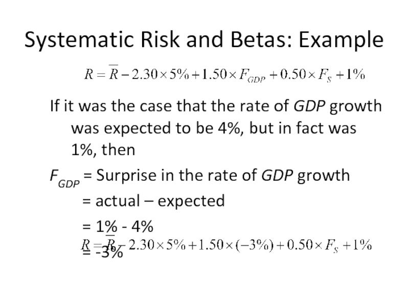
If it was the case that the
FGDP = Surprise in the rate of GDP growth
= actual – expected
= 1% - 4%
= -3%
Слайд 13Systematic Risk and Betas: Example
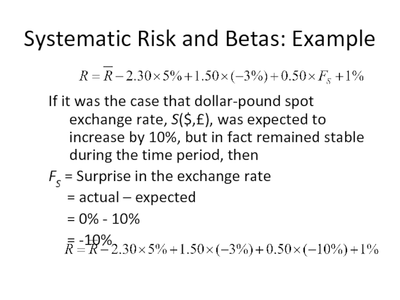
If it was the case that dollar-pound
FS = Surprise in the exchange rate
= actual – expected
= 0% - 10%
= -10%
Слайд 14Systematic Risk and Betas: Example
Finally, if it was the case that
Слайд 1511.4 Portfolios and Factor Models
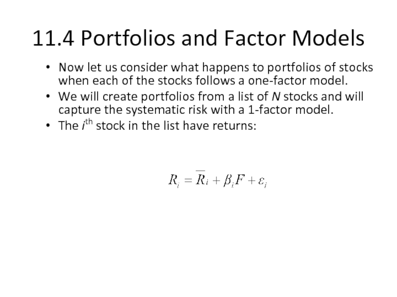
Now let us consider what happens to
We will create portfolios from a list of N stocks and will capture the systematic risk with a 1-factor model.
The ith stock in the list have returns:
Слайд 16
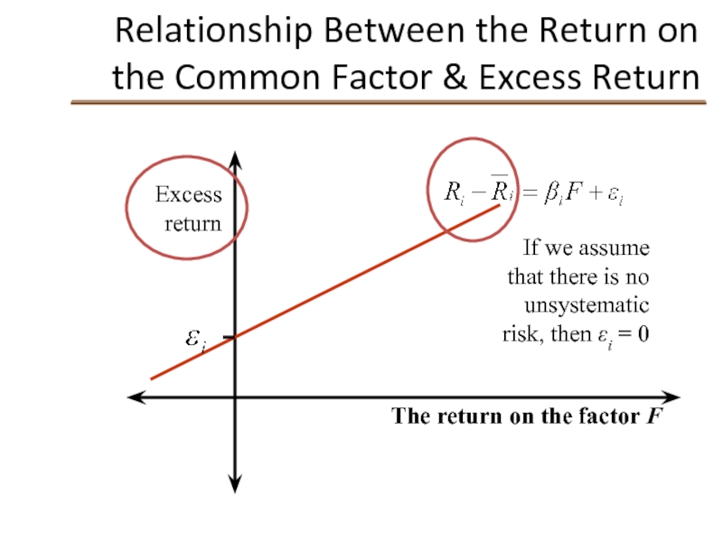
Relationship Between the Return on the Common Factor & Excess Return
Excess
The return on the factor F
If we assume that there is no unsystematic risk, then εi = 0
Слайд 17
Relationship Between the Return on the Common Factor & Excess Return
Excess
The return on the factor F
If we assume that there is no unsystematic risk, then εi = 0
Слайд 18
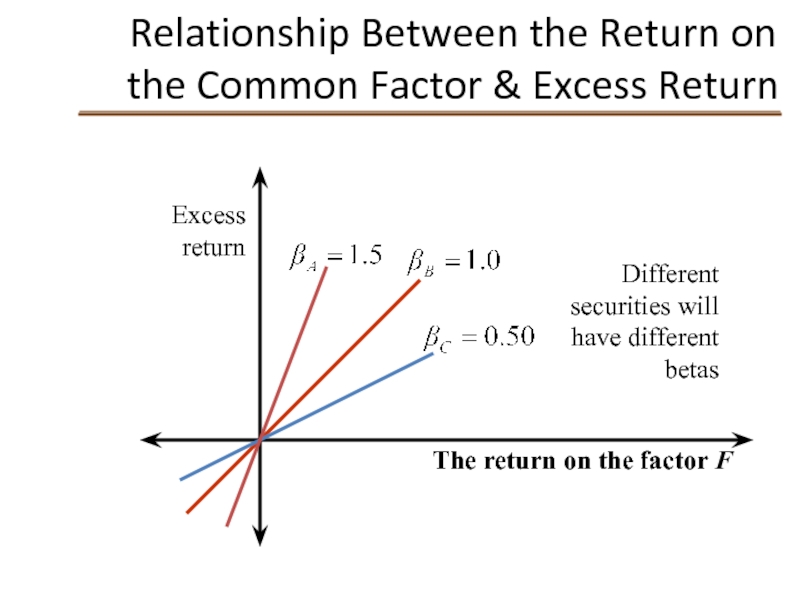
Relationship Between the Return on the Common Factor & Excess Return
Excess
The return on the factor F
Different securities will have different betas
Слайд 19Portfolios and Diversification
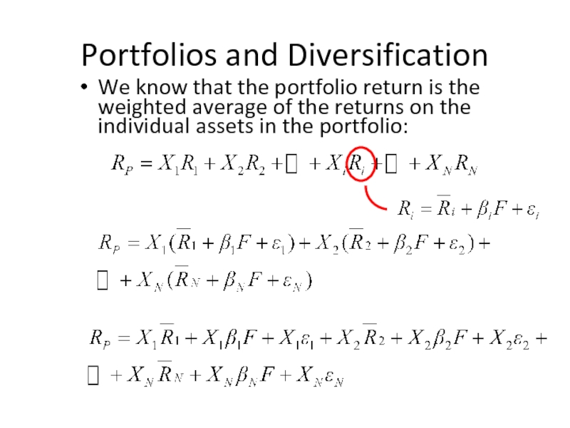
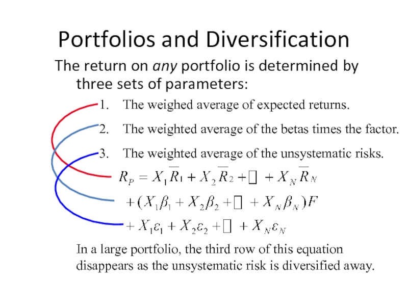
We know that the portfolio return is the weighted
Слайд 20Portfolios and Diversification
The return on any portfolio is determined by three
In a large portfolio, the third row of this equation disappears as the unsystematic risk is diversified away.
Слайд 21Portfolios and Diversification
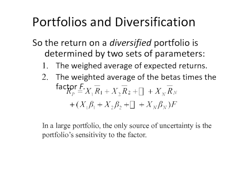
So the return on a diversified portfolio is determined
The weighed average of expected returns.
The weighted average of the betas times the factor F.
In a large portfolio, the only source of uncertainty is the portfolio’s sensitivity to the factor.
Слайд 2211.5 Betas and Expected Returns
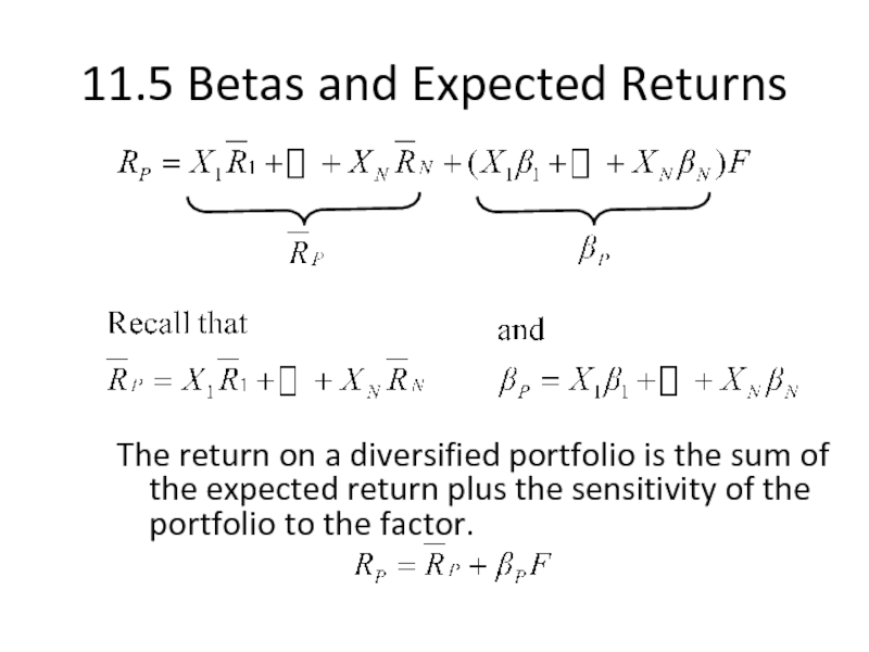
The return on a diversified portfolio is
Слайд 23Relationship Between β & Expected Return
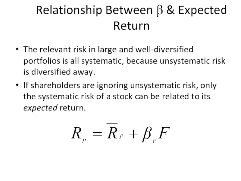
The relevant risk in large and
If shareholders are ignoring unsystematic risk, only the systematic risk of a stock can be related to its expected return.
Слайд 25
11.6 The Capital Asset Pricing Model and the Arbitrage Pricing Theory
APT
With APT it is possible for some individual stocks to be mispriced---not lie on the SML.
APT is more general in that it gets to an expected return and beta relationship without the assumption of the market portfolio.
APT can be extended to multifactor models.
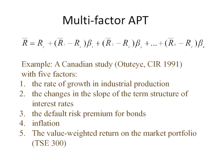
Слайд 26Multi-factor APT
Example: A Canadian study (Otuteye, CIR 1991)
with five factors:
the rate
the changes in the slope of the term structure of interest rates
the default risk premium for bonds
inflation
The value-weighted return on the market portfolio (TSE 300)
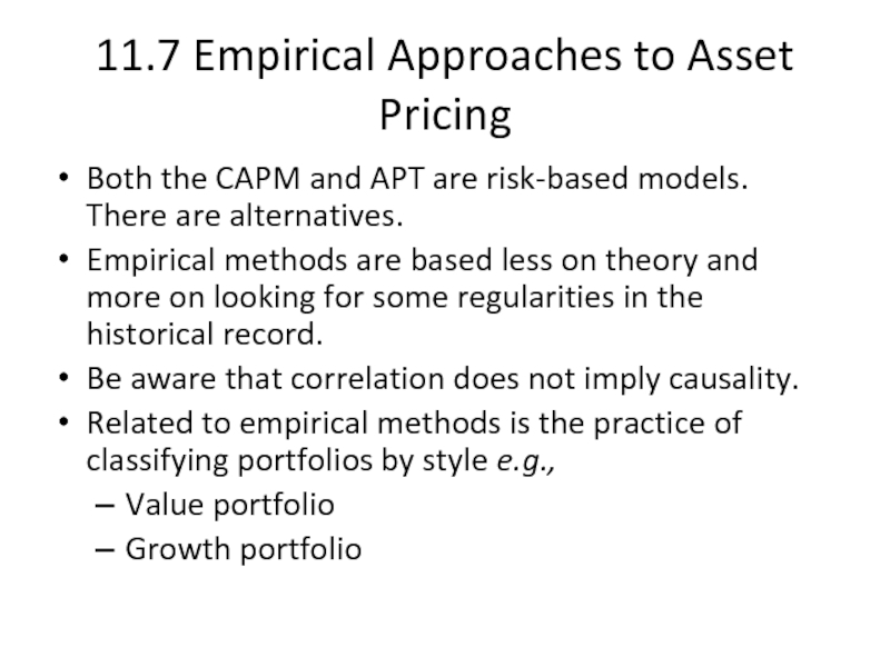
Слайд 2711.7 Empirical Approaches to Asset Pricing
Both the CAPM and APT are
Empirical methods are based less on theory and more on looking for some regularities in the historical record.
Be aware that correlation does not imply causality.
Related to empirical methods is the practice of classifying portfolios by style e.g.,
Value portfolio
Growth portfolio
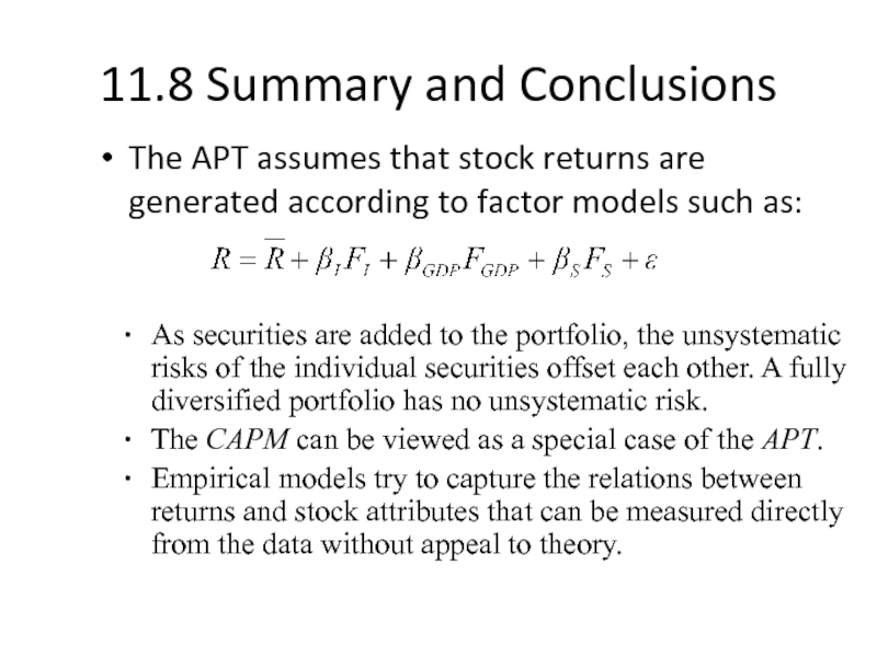
Слайд 2811.8 Summary and Conclusions
The APT assumes that stock returns are generated
As securities are added to the portfolio, the unsystematic risks of the individual securities offset each other. A fully diversified portfolio has no unsystematic risk.
The CAPM can be viewed as a special case of the APT.
Empirical models try to capture the relations between returns and stock attributes that can be measured directly from the data without appeal to theory.
