Darya Orlova
28 June, 2016
Darya Orlova
28 June, 2016

http://www.nist.gov/mml/bbd/bioassay/quantitative_flow_cytometry.cfm

The objective :


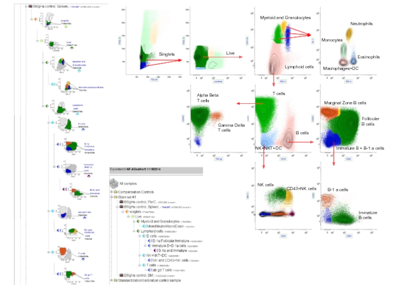
Follicular
B cells
Immature B + B-1 a cells


http://www.newsnshit.com/curse-of-dimensionality-interactive-demo/
Projection Pursuit

Goals:
quantitate differences between samples and provide a standard error
identify changes in joint expression of multiple markers
appropriately rank test samples based on the amount of deviation from controls
Quantification index allows biologically informative interpretation
 ≥ 0identity of indiscernibles d(x,y)")
How different are samples?
With respect to both the proportion of cells whose marker expression has changed and the magnitude of the change
Most of the current methods ask “Do samples differ?”


The biological interpretation of the EMD between two flow cytometry samples includes both the proportion of cells whose marker expression has changed
and the magnitude of the change
Earth mover's distance (EMD)

The optimal flow F between the source and destination signatures is determined by solving the linear programming problem.
EMD is then defined as a function of the optimal flow F=[fij] and the ground distance D=[dij]
Data were binned into the groups used in the signature according to (Roederer et al., 2001)
Earth mover's distance (EMD)
in terms of a linear programming problem
,…,(pm,wpm)} and Q={(q1,wq1),…,(qn,wqn)} where pi,qi are bin")
Surface CD203c in blood basophils after ex vivo stimulation with A. fumigatus (Af) allergen/extract (offending) or peanut (non offending) allergen. Gernez et al. J Cyst Fibros 11:502-10, 2012
Blood basophils from patients with ABPA are
hyper-responsive to stimulation by Af allergen
Antibiotics
Corticosteroids
Anti-fungal
medicines
 from allergic bronchopulmonary aspergillosis (ABPA) in CFSurface")
Total white blood cells (FSС-A/SSC-A)→singlets (FSС-A/FSC-H)→CD41a--live (CD41a/live/dead)→
Dump--CD123++ (CD3, CD66b, HLA-DR/CD123)


Antigen-antibody interactions on the surface of cells

Antibody*
Antibody*")
Mathematical model: kinetic of mean fluorescence
Reaction rate constant
Initial antibody concentration
n – binding sites per one bead/cell
K+
A0
;mean fluorescence value of cell Mathematical model:")
The total number of cells is the same for each histogram
 of FcgRIIIb receptors for different")
However, application of such rate constant approach is currently limited by the lack of measured binding rate constant values for most antigen-antibody pairs of interest and changes in experimental conditions (temperature, viscosity, fluorescent labels, etc.)

where η is the viscosity of the media, kB is the Boltzmann constant, T is the temperature; R1 and R2 are radii, N1 and N2 are valences of the first and second reactants, correspondingly.
The radius of antibody molecules can be estimated from the diffusion coefficient using Stokes–Einstein equation :
On the other hand, the diffusion coefficient of the molecule can be estimated using the known relationship between the diffusion coefficient (in cm2 s-1) and the molar mass (in Da), M, of a protein (in water at room temperature)


Electrical analogue
.Electrical analogue")
“Effective binding site” radius (b) can be calculated using the following expression:
where a and c are maximum length and maximum width (assuming a>c) of dominant amino acid residuals respectively (e.g. can be determine using HyperChem 7.5 software)


*


2. Assign all other clusters on this 2D plot either to cluster a or cluster b based on SC.
a
b
3. Now you have only two clusters A and B (for each possible 2D plot).
4. Calculate SC between A and B. Calculate % frequency for A and B. Now you can rank all possible 2D plots based on then SC and % frequency distribution between A and B. On the first place should be 2D plot with SC closest to 1 and % frequency distribution closest to 50/50 between A and B.
5. Pick A or B from most highly ranked 2D plot, project A(or B) to all possible 2D plots and proceed recursively with the same procedure (1-5).
 For each pair of clusters+their noise. Calculate % frequency for")

Если не удалось найти и скачать презентацию, Вы можете заказать его на нашем сайте. Мы постараемся найти нужный Вам материал и отправим по электронной почте. Не стесняйтесь обращаться к нам, если у вас возникли вопросы или пожелания:
Email: Нажмите что бы посмотреть
Это сайт презентаций, докладов, проектов, шаблонов в формате PowerPoint. Мы помогаем школьникам, студентам, учителям, преподавателям хранить и обмениваться учебными материалами с другими пользователями.


")


.")